Hi all, I am currently trying to implement faster rcnn using tensorflow. Due to the limitations of the machine I am working on I can only use tensorflow 1.15. However, the model that I wanted to originally use as a feature extractor is built with Keras and tf2. Now I’m left wondering what I’m supposed to use to build the model for the feature extractor if I can’t use Keras. Should I just try to implement the inception resnet model by myself? Any help would be appreciated
I’m trying to create a model to predict latitude and longitude from an image. However, my loss does not decrease at all during training, and the predictions are very far off.
Is what I’m doing realistically possible? And if so, how can I make my model more accurate?
NVIDIA announced TensorRT 8.0 which brings BERT-Large inference latency down to 1.2 ms with new optimizations.
Today, NVIDIA announced TensorRT 8.0 which brings BERT-Large inference latency down to 1.2 ms with new optimizations. This version also delivers 2x the accuracy for INT8 precision with Quantization Aware Training, and significantly higher performance through support for Sparsity, which was introduced in Ampere GPUs.
TensorRT is an SDK for high-performance deep learning inference that includes an inference optimizer and runtime that delivers low latency and high throughput. TensorRT is used across industries such as Healthcare, Automotive, Manufacturing, Internet/Telecom services, Financial Services, Energy, and has been downloaded nearly 2.5 million times.
There have been several kinds of new transformer-based models used across conversational AI. New generalized optimizations in TensorRT can accelerate all such models reducing inference time to half the time vs TensorRT 7.
Highlights from this version include:
BERT Inference in 1.2 ms with new transformer optimizations
Achieve accuracy equivalent to FP32 with INT8 precision using Quantization Aware Training
Introducing Sparsity support for faster inference on Ampere GPUs
One of the biggest social media platforms in China, WeChat accelerates its search using TensorRT serving 500M users a month.
“We have implemented TensorRT-and-INT8 QAT-based model inference acceleration to accelerate core tasks of WeChat Search such as Query Understanding and Results Ranking. The conventional limitation of NLP model complexity has been broken-through by our solution with GPU + TensorRT, and BERT/Transformer can be fully integrated in our solution. In addition, we have achieved significant reduction (70%) in allocated computational resources using superb performance optimization methods. ” – Huili/Raccoonliu/Dickzhu, WeChat Search
NVIDIA today launched TensorRT™ 8, the eighth generation of the company’s AI software, which slashes inference time in half for language queries — enabling developers to build the world’s best-performing search engines, ad recommendations and chatbots and offer them from the cloud to the edge.
The final push for the hat trick came down to the wire. Five minutes before the deadline, the team submitted work in its third and hardest data science competition of the year in recommendation systems. Called RecSys, it’s a relatively new branch of computer science that’s spawned one of the most widely used applications in Read article >
Today, NVIDIA is releasing TensorRT 8.0, which introduces many transformer optimizations. With this post update, we present the latest TensorRT optimized BERT sample and its inference latency benchmark on A30 GPUs. Using the optimized sample, you can execute different batch sizes for BERT-base or BERT-large within the 10 ms latency budget for conversational AI applications.
This post was originally published in August 2019 and has been updated for NVIDIA TensorRT 8.0.
Large-scale language models (LSLMs) such as BERT, GPT-2, and XL-Net have brought exciting leaps in accuracy for many natural language processing (NLP) tasks. Since its release in October 2018, BERT (Bidirectional Encoder Representations from Transformers), with all its many variants, remains one of the most popular language models and still delivers state-of-the-art accuracy.
BERT provided a leap in accuracy for NLP tasks that brought high-quality, language-based services within the reach of companies across many industries. To use the model in production, you must consider factors such as latency and accuracy, which influences end-user satisfaction with a service. BERT requires significant compute during inference due to its 12/24-layer stacked, multihead attention network. This has posed a challenge for companies to deploy BERT as part of real-time applications.
Today, NVIDIA is releasing version 8 of TensorRT, which brings the inference latency of BERT-Large down to 1.2 ms on NVIDIA A100 GPUs with new optimizations on transformer-based networks. New generalized optimizations in TensorRT can accelerate all such models, reducing inference time to half the time compared to TensorRT 7.
TensorRT
TensorRT is a platform for high-performance, deep learning inference, which includes an optimizer and runtime that minimizes latency and maximizes throughput in production. With TensorRT, you can optimize models trained in all major frameworks, calibrate for lower precision with high accuracy, and finally deploy in production.
All the code for achieving this performance with BERT is being released as open source in this NVIDIA/TensorRT GitHub repo. We have optimized the Transformer layer, which is a fundamental building block of the BERT encoder so that you can adapt these optimizations to any BERT-based NLP task. BERT is applied to an expanding set of speech and NLP applications beyond conversational AI, all of which can take advantage of these optimizations.
Question answering (QA) or reading comprehension is a popular way to test the ability of models to understand the context. The SQuAD leaderboard tracks the top performers for this task, for a dataset and test set that they provide. There has been rapid progress in QA ability in the last few years, with global contributions from academia and companies.
In this post, we demonstrate how to create a simple QA application using Python, powered by TensorRT-optimized BERT code that NVIDIA released today. The example provides an API to input passages and questions, and it returns responses generated by the BERT model.
Here’s a brief review of the steps to perform training and inference using TensorRT for BERT.
BERT training and inference pipeline
A major problem faced by NLP researchers and developers is scarcity of high-quality labeled training data for their specific NLP task. To overcome the problem of learning a model for the task from scratch, breakthroughs in NLP use the vast amounts of unlabeled text and break the NLP task into two parts:
Learning to represent the meaning of words, the relationship between them, that is, building up a language model using auxiliary tasks and a large corpus of text
Specializing the language model to the actual task by augmenting the language model with a relatively small, task-specific network that is trained in a supervised manner.
These two stages are typically referred to as pretraining and fine-tuning. This paradigm enables the use of the pretrained language model to a wide range of tasks without any task-specific change to the model architecture. In this example, BERT provides a high-quality language model that is fine-tuned for QA but suitable for other tasks such as sentence classification and sentiment analysis.
You can either start with the pretrained checkpoints available online or pretrain BERT on your own custom corpus (Figure 1). You can also initialize pretraining from a checkpoint and then continue training on custom data.
Figure 1. Generating BERT TensorRT engine from pretrained checkpoints
Pretraining with custom or domain-specific data may yield interesting results, for example BioBert. However, it is computationally intensive and requires a massively parallel compute infrastructure to complete within a reasonable amount of time. GPU-enabled, multinode training is an ideal solution for such scenarios. For more information about how NVIDIA developers were able to train BERT in less than an hour, see Training BERT with GPUs.
In the fine-tuning step, the task-specific network based on the pretrained BERT language model is trained using the task-specific training data. For QA, this is (paragraph, question, answer) triples. Compared to pretraining, fine-tuning is generally far less computationally demanding.
To perform inference using a QA neural network:
Create a TensorRT engine by passing the fine-tuned weights and network definition to the TensorRT builder.
Start the TensorRT runtime with this engine.
Feed a passage and a question to the TensorRT runtime and receive as output the answer predicted by the network.
Figure 2 shows the entire workflow.
Figure 2. Workflow to perform inference with TensorRT runtime engine for BERT QA task
Run the sample!
Set up your environment to perform BERT inference with the following steps:
Create a Docker image with the prerequisites.
Build the TensorRT engine from the fine-tuned weights.
Perform inference given a passage and query.
We use scripts to perform these steps, which you can find in the TensorRT BERT sample repo. While we describe several options that you can pass to each script, to get started quickly, you could also run the following code example:
 # Clone the TensorRT repository and navigate to BERT demo directory
 git clone --recursive https://github.com/NVIDIA/TensorRT && cd TensorRT

 # Create and launch the Docker image
 # Here we assume the following:
 #  - the os being ubuntu-18.04 (see below for other supported versions)
 #  - cuda version is 11.3.1
 bash docker/build.sh --file docker/ubuntu-18.04.Dockerfile --tag tensorrt-ubuntu18.04-cuda11.3 --cuda 11.3.1

 # Run the Docker container just created
 bash docker/launch.sh --tag tensorrt-ubuntu18.04-cuda11.3 --gpus all

 # cd into the BERT demo folder
 cd $TRT_OSSPATH/demo/BERT

 # Download the BERT model fine-tuned checkpoint
 bash scripts/download_model.sh

 # Build the TensorRT runtime engine.
 # To build an engine, use the builder.py script.
 mkdir -p engines && python3 builder.py -m models/fine-tuned/bert_tf_ckpt_large_qa_squad2_amp_128_v19.03.1/model.ckpt -o engines/bert_large_128.engine -b 1 -s 128 --fp16 -c models/fine-tuned/bert_tf_ckpt_large_qa_squad2_amp_128_v19.03.1
This last command builds an engine with a maximum batch size of 1 (-b 1), and sequence length of 128 (-s 128) using mixed precision (--fp16) and the BERT Large SQuAD v2 FP16 Sequence Length 128 checkpoint (-c models/fine-tuned/bert_tf_ckpt_large_qa_squad2_amp_128_v19.03.1).
Now, give it a passage and see how much information it can decipher by asking a few questions.
python3 inference.py -e engines/bert_large_128.engine -p "TensorRT is a high performance deep learning inference platform that delivers low latency and high throughput for apps such as recommenders, speech and image/video on NVIDIA GPUs. It includes parsers to import models, and plugins to support novel ops and layers before applying optimizations for inference. Today NVIDIA is open-sourcing parsers and plugins in TensorRT so that the deep learning community can customize and extend these components to take advantage of powerful TensorRT optimizations for your apps." -q "What is TensorRT?" -v models/fine-tuned/bert_tf_ckpt_large_qa_squad2_amp_128_v19.03.1/vocab.txt
The result of this command should be something similar to the following:
Passage: TensorRT is a high performance deep learning inference platform that delivers low latency and high throughput for apps such as recommenders, speech and image/video on NVIDIA GPUs. It includes parsers to import models, and plugins to support novel ops and layers before applying optimizations for inference. Today NVIDIA is open-sourcing parsers and plugins in TensorRT so that the deep learning community can customize and extend these components to take advantage of powerful TensorRT optimizations for your apps.
Question: What is TensorRT?
Answer: 'a high performance deep learning inference platform'
Given the same passage with a different question, you should get the following result:
Question: What is included in TensorRT?
Answer: 'parsers to import models, and plugins to support novel ops and layers before applying optimizations for inference'
The answers provided by the model are accurate based on the text of the passage that was provided. The sample uses FP16 precision for performing inference with TensorRT. This helps achieve the highest performance possible on Tensor Cores in NVIDIA GPUs. In our tests, we measured the accuracy of TensorRT to be comparable to in-framework inference with FP16 precision.
Script options
Here are the options available with the scripts. The docker/build.sh script builds the docker image using the Dockerfile supplied in the docker folder. It installs all necessary packages, depending on the OS you are selecting as Dockerfile. For this post, we used ubuntu-18.04 but dockerfiles for ubuntu-16.04 and ubuntu-20.04 are also provided.
After creating and running the environment, download fine-tuned weights for BERT. Note that you do not need the pretrained weights to create the TensorRT engine (just the fine-tuned weights). Along with the fine-tuned weights, use the associated configuration file, which specifies parameters such as number of attention heads, number of layers, and the vocab.txt file, which contains the learned vocabulary from the training process. These are packaged with the fine-tuned model downloaded from NGC; download them using the download_model.sh script. As part of this script, you can specify the set of fine-tuned weights for the BERT model to download. The command-line parameters control the exact BERT model to be used later for model building and inference:
sh download_model.sh [tf|pyt] [base|large|megatron-large] [128|384] [v2|v1_1] [sparse] [int8-qat]
 tf | pyt tensorflow or pytorch version
 base | large | megatron-large - determine whether to download a BERT-base or BERT-large or megatron model to optimize
 128 | 384 - determine whether to download a BERT model for sequence length 128 or 384
 v2 | v1_1, fine-tuned on squad2 or squad1.1
 sparse, download sparse version
 int8-qat, download int8 weights
Examples:
# Running with default parametersbash download_model.sh# Running with custom parameters (BERT-large, FP32 fine-tuned weights, 128 sequence length)sh download_model.sh large tf fp32 128
This script by default downloads fine-tuned TensorFlow BERT-large, with FP16 precision and a sequence length of 128. In addition to the fine-tuned model, you use the configuration file, enumerating model parameters and the vocabulary file used to convert BERT model output to a textual answer.
Next, you can build the TensorRT engine and use it for a QA example, that is, inference. The script builder.py builds the TensorRT engine for inference based on the downloaded BERT fine-tuned model.
Make sure that the sequence length provided to the following script matches the sequence length of the model that was downloaded.
   -h, --help    show this help message and exit
   -m CKPT, --ckpt CKPT  The checkpoint file basename, e.g.:
 basename(model.ckpt-766908.data-00000-of-00001) is model.ckpt-766908 (default: None)
   -x ONNX, --onnx ONNX  The ONNX model file path. (default: None)
   -pt PYTORCH, --pytorch PYTORCH
             The PyTorch checkpoint file path. (default: None)
   -o OUTPUT, --output OUTPUT
             The bert engine file, ex bert.engine (default: bert_base_384.engine)
   -b BATCH_SIZE, --batch-size BATCH_SIZE
 Batch size(s) to optimize for.
 The engine will be usable with any batch size below this, but may not be optimal for smaller sizes. Can be specified multiple times to optimize for more than one batch size.(default: [])
   -s SEQUENCE_LENGTH, --sequence-length SEQUENCE_LENGTH
             Sequence length of the BERT model (default: [])
   -c CONFIG_DIR, --config-dir CONFIG_DIR
 The folder containing the bert_config.json,
 which can be downloaded e.g. from https://github.com/google-research/bert#pre-trained-models (default: None)
   -f, --fp16    Indicates that inference should be run in FP16 precision
             (default: False)
   -i, --int8    Indicates that inference should be run in INT8 precision
             (default: False)
   -t, --strict  Indicates that inference should be run in strict precision mode
             (default: False)
   -w WORKSPACE_SIZE, --workspace-size WORKSPACE_SIZE Workspace size in MiB for
             building the BERT engine (default: 1000)
   -j SQUAD_JSON, --squad-json SQUAD_JSON
 squad json dataset used for int8 calibration (default: squad/dev-v1.1.json)
   -v VOCAB_FILE, --vocab-file VOCAB_FILE
 Path to file containing entire understandable vocab (default: ./pre-trained_model/uncased_L-24_H-1024_A-16/vocab.txt)
   -n CALIB_NUM, --calib-num CALIB_NUM
             calibration batch numbers (default: 100)
   -p CALIB_PATH, --calib-path CALIB_PATH
             calibration cache path (default: None)
   -g, --force-fc2-gemm
             Force use gemm to implement FC2 layer (default: False)
   -iln, --force-int8-skipln
 Run skip layernorm with INT8 (FP32 or FP16 by default) inputs and output (default: False)
   -imh, --force-int8-multihead
 Run multi-head attention with INT8 (FP32 or FP16 by default) input and output (default: False)
   -sp, --sparse         Indicates that model is sparse (default: False)
   -tcf TIMING_CACHE_FILE, --timing-cache-file TIMING_CACHE_FILE
 Path to tensorrt build timeing cache file, only available for tensorrt 8.0 and later (default: None)
You should now have a TensorRT engine, engines/bert_large_128.engine, to use in the inference.py script for QA.
Later in this post, we describe the process to build the TensorRT engine. You can now provide a passage and a query to inference.py and see if the model is able to answer your queries correctly.
There are few ways to interact with the inference script:
The passage and question can be provided as command-line arguments using the –passage and –question flags.
They can be passed in from a given file using the –passage_file and –question_file flags.
If neither of these flags are given during execution, you are prompted to enter the passage and question after the execution has begun.
Here are the parameters for the inference.py script:
This script uses a prebuilt TensorRT BERT QA engine to answer a question based on the provided passage.
Here are the optional arguments:
   -h, --help            show this help message and exit
   -e ENGINE, --engine ENGINE
                         Path to BERT TensorRT engine
   -b BATCH_SIZE, --batch-size BATCH_SIZE
                         Batch size for inference.
   -p [PASSAGE [PASSAGE ...]], --passage [PASSAGE [PASSAGE ...]]
                         Text for paragraph/passage for BERT QA
   -pf PASSAGE_FILE, --passage-file PASSAGE_FILE
                         File containing input passage
   -q [QUESTION [QUESTION ...]], --question [QUESTION [QUESTION ...]]
                         Text for query/question for BERT QA
   -qf QUESTION_FILE, --question-file QUESTION_FILE
                         File containing input question
   -sq SQUAD_JSON, --squad-json SQUAD_JSON
                         SQuAD json file
   -o OUTPUT_PREDICTION_FILE, --output-prediction-file OUTPUT_PREDICTION_FILE
                         Output prediction file for SQuAD evaluation
   -v VOCAB_FILE, --vocab-file VOCAB_FILE
                         Path to file containing entire understandable vocab
   -s SEQUENCE_LENGTH, --sequence-length SEQUENCE_LENGTH
                         The sequence length to use. Defaults to 128
   --max-query-length MAX_QUERY_LENGTH
                         The maximum length of a query in number of tokens.
                         Queries longer than this will be truncated
   --max-answer-length MAX_ANSWER_LENGTH
                         The maximum length of an answer that can be generated
   --n-best-size N_BEST_SIZE
                         Total number of n-best predictions to generate in the
                         nbest_predictions.json output file
   --doc-stride DOC_STRIDE
                         When splitting up a long document into chunks, what
                         stride to take between chunks
BERT inference with TensorRT
For a step-by-step description and walkthrough of the inference process, see the Python script inference.py and the detailed Jupyter notebook inference.ipynb in the sample folder. Here are a few key parameters and concepts for performing inference with TensorRT.
BERT, or more specifically, the encoder layer, uses the following parameters to govern its operation:
Batch size
Sequence Length
Number of attention heads
The value of these parameters, which depend on the BERT model chosen, are used to set the configuration parameters for the TensorRT plan file (execution engine).
For each encoder, also specify the number of hidden layers and the attention head size. You can also read all the earlier parameters from the TensorFlow checkpoint file.
As the BERT model we are using has been fine-tuned for a downstream task of QA on the SQuAD dataset, the output for the network (that is, the output fully connected layer) is a span of text where the answer appears in the passage, referred to as h_output in the sample. After you generate the TensorRT engine, you can serialize it and use it later with TensorRT runtime.
During inference, you perform memory copies from CPU to GPU and the reverse asynchronously to get tensors into and out of the GPU memory, respectively. Asynchronous memory copy operation hides the latency of memory transfer by overlapping computations with memory copy operation between device and host. Figure 3 shows the asynchronous memory copies and kernel execution.
Figure 3. TensorRT Runtime process
The inputs to the BERT model (Figure 3) include the following:
input_ids: tensor with token ids of paragraph concatenated along with question that is used as input for inference
segment_ids: distinguishes between passage and question
input_mask: indicates which elements in the sequence are tokens, and which ones are padding elements
The outputs (start_logits and end_logits) represent the span of the answer, which the network predicts inside the passage based on the question.
Benchmarking BERT inference performance
BERT can be applied both for online and offline use cases. Online NLP applications, such as conversational AI, place tight latency budgets during inference. Several models need to execute in a sequence in response to a single user query. When used as a service, the total time a customer experiences includes compute time as well as input and output network latency. Longer times lead to a sluggish performance and a poor customer experience.
While the exact latency available for a single model can vary by application, several real-time applications need the language model to execute in under 10 ms.
Using an NVIDIA Ampere Architecture A100 GPU, BERT-Large optimized with TensorRT 8 can perform inference in 1.2ms for a QA task similar to that available in SQuAD with batch size = 1 and sequence length = 128.
Using the TensorRT optimized sample, you can execute different batch sizes for BERT-base or BERT-large within the 10 ms latency budget. For example, the latency for inference on a BERT-Large model with sequence length = 384 batch size = 1 on A30 with TensorRT8 was 3.62ms. The same model, sequence length =384 with highly optimized code on a CPU-only platform (**) for batch size = 1 was 76ms.
Figure 4. Compute latency in milliseconds for executing BERT-large on an NVIDIA A30 GPU vs. a CPU-only server
The performance measures the compute-only latency time for executing the network on a QA task between passing tensors as input and gathering logits as output. You can find the code used to benchmark the sample in the script scripts/inference_benchmark.sh in the repo.
Summary
NVIDIA is releasing TensorRT 8.0, which makes it possible to perform BERT inference in 0.74ms on A30 GPUs. The code for benchmarking inference on BERT is available as a sample in the TensorRT open-source repo.
This post gives an overview of how to use the TensorRT sample and performance results. We further describe a workflow of how to use the BERT sample as part of a simple application and Jupyter notebook where you can pass a paragraph and ask questions related to it. The new optimizations and performance achievable makes it practical to use BERT in production for applications with tight latency budgets, such as conversational AI.
We are always looking for new ideas for new examples and applications to share. What NLP applications do you use BERT for and what examples would you like to see from us in the future?
CPU-only specifications: Gold 6240@2.60GHz 3.9GHz Turbo (Cascade Lake) HT Off, Single node, Single Socket, Number of CPU Threads = 18, Data=Real, Batch Size=1; Sequence Length=128; nireq=1; Precision=FP32; Data=Real; OpenVINO 2019 R2
GPU-server specification: Gold 6140@2GHz 3.7GHz Turbo (Skylake) HT On, Single node, Dual Socket, Number of CPU Threads = 72, T4 16GB, Driver Version 418.67 (r418_00), BERT-base, Batch Size=1; Number of heads = 12, Size per head = 64; 12 layers; Sequence Length=128; Precision=FP16; XLA=Yes; Data=Real; TensorRT 5.1
(**)
CPU-only specifications: Platinum 8380H@2.90GHz to 4.3 GHz Turbo (Cooper Lake) HT Off, Single node, Single Socket, Number of CPU Threads = 28, BERT-Large, Data=Real, Batch Size=1; Sequence Length=384; nireq=1; Precision=INT8; Data=Real; OpenVINO 2021 R3
GPU-server specification: AMD EPYC 7742@2.25GHz 3.4GHz Turbo (Rome) HT Off, Single node, Number of CPU Threads = 64, A30(GA100) 1*24258 MiB 1*56 SM, Driver Version 470.29 (r470_00), BERT-Large, Batch Size=1; Sequence Length=384; Precision=INT8; TensorRT 8.0
The NVIDIA Merlin and KGMON team earned 1st place in the RecSys Challenge 2021 by effectively predicting the probability of user engagement within a dynamic environment and providing fair recommendations on a multi-million point dataset.
The NVIDIA Merlin and KGMON team earned 1st place in the RecSys Challenge 2021 by effectively predicting the probability of user engagement within a dynamic environment and providing fair recommendations on a multi-million point dataset. Twitter sponsored the RecSys Challenge 2021, curated the challenge’s multi-goal optimization requirements to mirror the real world, and provided multi-million data points each day over the course of the challenge for the teams to work with. NVIDIA’s win for a second year in a row reaffirms NVIDIA’s continued commitment to democratize and streamline recommender workflows.
NVIDIA Merlin Team Weaves Industry Engagement and Learnings Into Software Product
Billions of people are online. Each moment online represents an opportunity for a person to engage with a recommender while reading news, streaming entertainment, shopping, or engaging with social media. Twitter, as a single social media platform, reports an average of 199 million monetizable daily active users that engage within its dynamic environment. The RecSys Challenge 2021 reflects how providing quality recommendations that span millions of data points is extremely challenging. The Merlin team builds open source software designed to help machine learning engineers and data scientists tackle these problems and more. The team also leveraged their skills and experience building Merlin software to win the RecSys Challenge 2021. The challenge also provided insights and opportunities that feed back into Merlin, helping to continuously improve the product. For example, operators used to win last year’s RecSys Challenge 2020 were woven into a product release. This is particularly impactful when working with the Kaggle Grandmasters Of NVIDIA (KGMON) team who are regular collaborators with the Merlin team on recommendation competitions and who bring insight from hundreds of kaggle competition wins. The Merlin team’s hands-on engagement coupled with feedback from Merlin’s early adopters, is vital for reaffirming NVIDIA’s commitment of democratizing the building and accelerating of recommenders.
Editor’s note: Feature image includes just a few of NVIDIA team members that participated in the challenge (clockwise from upper left): Bo Liu, Benedikt Schifferer, Gilberto Titericz and Chris Deotte.
This post was updated July 20, 2021 to reflect NVIDIA TensorRT 8.0 updates. NVIDIA TensorRT is an SDK for deep learning inference. TensorRT provides APIs and parsers to import trained models from all major deep learning frameworks. It then generates optimized runtime engines deployable in the datacenter as well as in automotive and embedded environments. … Continued
This post was updated July 20, 2021 to reflect NVIDIA TensorRT 8.0 updates.
NVIDIA TensorRT is an SDK for deep learning inference. TensorRT provides APIs and parsers to import trained models from all major deep learning frameworks. It then generates optimized runtime engines deployable in the datacenter as well as in automotive and embedded environments.
This post provides a simple introduction to using TensorRT. You learn how to deploy a deep learning application onto a GPU, increasing throughput and reducing latency during inference. It uses a C++ example to walk you through converting a PyTorch model into an ONNX model and importing it into TensorRT, applying optimizations, and generating a high-performance runtime engine for the datacenter environment.
TensorRT supports both C++ and Python; if you use either, this workflow discussion could be useful. If you prefer to use Python, see Using the Python API in the TensorRT documentation.
Deep learning applies to a wide range of applications such as natural language processing, recommender systems, image, and video analysis. As more applications use deep learning in production, demands on accuracy and performance have led to strong growth in model complexity and size.
Safety-critical applications such as automotive place strict requirements on throughput and latency expected from deep learning models. The same holds true for some consumer applications, including recommendation systems.
TensorRT is designed to help deploy deep learning for these use cases. With support for every major framework, TensorRT helps process large amounts of data with low latency through powerful optimizations, use of reduced precision, and efficient memory use.
To follow along with this post, you need a computer with a CUDA-capable GPU or a cloud instance with GPUs and an installation of TensorRT. On Linux, the easiest place to get started is by downloading the GPU-accelerated PyTorch container with TensorRT integration from the NVIDIA Container Registry (on NGC). The link will have an updated version of the container, but to make sure that this tutorial works properly, we specify the version used for this post:
Because you use TensorRT 8 in this walkthrough, you must upgrade it in the container. The next step is to download the .deb package for TensorRT 8 (CUDA 11.0, Ubuntu 18.04), and install the following requirements:
# Export absolute path to directory hosting TRT8.deb
export TRT_DEB_DIR_PATH=$HOME/trt_release  # Change this path to where you’re keeping your .deb file

# Run container
docker run --rm --gpus all -ti --volume $TRT_DEB_DIR_PATH:/workspace/trt_release --net host nvcr.io/nvidia/pytorch:20.07-py3

# Update TensorRT version to 8
dpkg -i nv-tensorrt-repo-ubuntu1804-cuda11.0-trt8.0.0.3-ea-20210423_1-1_amd64.deb
apt-key add /var/nv-tensorrt-repo-ubuntu1804-cuda11.0-trt8.0.0.3-ea-20210423/7fa2af80.pub

apt-get update
apt-get install -y libnvinfer8 libnvinfer-plugin8 libnvparsers8 libnvonnxparsers8
apt-get install -y libnvinfer-bin libnvinfer-dev libnvinfer-plugin-dev libnvparsers-dev
apt-get install -y tensorrt

# Verify TRT 8.0.0 installation
dpkg -l | grep TensorRT
Simple TensorRT example
Following are the four steps for this example application:
Convert the pretrained image segmentation PyTorch model into ONNX.
Import the ONNX model into TensorRT.
Apply optimizations and generate an engine.
Perform inference on the GPU.
Importing the ONNX model includes loading it from a saved file on disk and converting it to a TensorRT network from its native framework or format. ONNX is a standard for representing deep learning models enabling them to be transferred between frameworks.
Many frameworks such as Caffe2, Chainer, CNTK, PaddlePaddle, PyTorch, and MXNet support the ONNX format. Next, an optimized TensorRT engine is built based on the input model, target GPU platform, and other configuration parameters specified. The last step is to provide input data to the TensorRT engine to perform inference.
The application uses the following components in TensorRT:
ONNX parser: Takes a converted PyTorch trained model into the ONNX format as input and populates a network object in TensorRT.
Builder: Takes a network in TensorRT and generates an engine that is optimized for the target platform.
Engine: Takes input data, performs inferences, and emits inference output.
Logger: Associated with the builder and engine to capture errors, warnings, and other information during the build and inference phases.
Convert the pretrained image segmentation PyTorch model into ONNX
After you have successfully installed the PyTorch container from the NGC registry and upgraded it with TensorRT 8.0, run the following commands to download everything needed to run this sample application (example code, test input data, and reference outputs). Then, update the dependencies and compile the application with the makefile provided.
>> sudo apt-get install libprotobuf-dev protobuf-compiler # protobuf is a prerequisite library
>> git clone --recursive https://github.com/onnx/onnx.git # Pull the ONNX repository from GitHub
>> cd onnx
>> mkdir build && cd build
>> cmake .. # Compile and install ONNX
>> make # Use the ‘-j’ option for parallel jobs, for example, ‘make -j $(nproc)’
>> make install
>> cd ../..
>> git clone https://github.com/parallel-forall/code-samples.git
>> cd code-samples/posts/TensorRT-introduction
Modify $TRT_INSTALL_DIR in the Makefile.
>> make clean && make # Compile the TensorRT C++ code
>> cd ..
>> wget https://developer.download.nvidia.com/devblogs/speeding-up-unet.7z // Get the ONNX model and test the data
>> sudo apt install p7zip-full
>> 7z x speeding-up-unet.7z # Unpack the model data into the unet folder
>> cd unet
>> python create_network.py #Inside the unet folder, it creates the unet.onnx file
Convert the PyTorch-trained UNet model into ONNX, as shown in the following code example:
Next, prepare the input data for inference. Download all images from the Kaggle directory. Copy to the /unet directory any three images that don’t have _mask in their filename and the utils.py file from the brain-segmentation-pytorch repository. Prepare three images to be used as input data later in this post. To prepare the input_0. pb and ouput_0. pb files for use later, run the following code example:
import torch
import argparse
import numpy as np
from torchvision import transforms
from skimage.io import imread
from onnx import numpy_helper
from utils import normalize_volume
def main(args):
    model = torch.hub.load('mateuszbuda/brain-segmentation-pytorch', 'unet',
      in_channels=3, out_channels=1, init_features=32, pretrained=True)
    model.train(False)

    filename = args.input_image
    input_image = imread(filename)
    input_image = normalize_volume(input_image)
    input_image = np.asarray(input_image, dtype='float32')

    preprocess = transforms.Compose([
      transforms.ToTensor(),
    ])
    input_tensor = preprocess(input_image)
    input_batch = input_tensor.unsqueeze(0)

    tensor1 = numpy_helper.from_array(input_batch.numpy())
    with open(args.input_tensor, 'wb') as f:
        f.write(tensor1.SerializeToString())
    if torch.cuda.is_available():
        input_batch = input_batch.to('cuda')
        model = model.to('cuda')
    with torch.no_grad():
        output = model(input_batch)

    tensor = numpy_helper.from_array(output[0].cpu().numpy())
    with open(args.output_tensor, 'wb') as f:
        f.write(tensor.SerializeToString())
if __name__=='__main__':
    parser = argparse.ArgumentParser()
    parser.add_argument('--input_image', type=str)
    parser.add_argument('--input_tensor', type=str, default='input_0.pb')
    parser.add_argument('--output_tensor', type=str, default='output_0.pb')
    args=parser.parse_args()
    main(args)
To generate processed input data for inference, run the following commands:
>> pip install medpy #dependency for utils.py file
>> mkdir test_data_set_0
>> mkdir test_data_set_1
>> mkdir test_data_set_2
>> python prepareData.py --input_image your_image1 --input_tensor test_data_set_0/input_0.pb --output_tensor test_data_set_0/output_0.pb   # This creates input_0.pb and output_0.pb
>> python prepareData.py --input_image your_image2 --input_tensor test_data_set_1/input_0.pb --output_tensor test_data_set_1/output_0.pb   # This creates input_0.pb and output_0.pb
>> python prepareData.py --input_image your_image3 --input_tensor test_data_set_2/input_0.pb --output_tensor test_data_set_2/output_0.pb   # This creates input_0.pb and output_0.pb
That’s it, you have the input data ready to perform inference.
Import the ONNX model into TensorRT, generate the engine, and perform inference
Run the sample application with the trained model and input data passed as inputs. The data is provided as an ONNX protobuf file. The sample application compares output generated from TensorRT with reference values available as ONNX .pb files in the same folder and summarizes the result on the prompt.
It can take a few seconds to import the UNet ONNX model and generate the engine. It also generates the output image in the portable gray map (PGM) format as output.pgm.
 >> cd to code-samples/posts/TensorRT-introduction-updated
 >> ./simpleOnnx path/to/unet/unet.onnx fp32 path/to/unet/test_data_set_0/input_0.pb # The sample application expects output reference values in path/to/unet/test_data_set_0/output_0.pb
 ...
 ...
 : --------------- Timing Runner: Conv_40 + Relu_41 (CaskConvolution)
 : Conv_40 + Relu_41 Set Tactic Name: volta_scudnn_128x128_relu_exp_medium_nhwc_tn_v1 Tactic: 861694390046228376
 : Tactic: 861694390046228376 Time: 0.237568
 ...
 : Conv_40 + Relu_41 Set Tactic Name: volta_scudnn_128x128_relu_exp_large_nhwc_tn_v1 Tactic: -3853827649136781465
 : Tactic: -3853827649136781465 Time: 0.237568
 : Conv_40 + Relu_41 Set Tactic Name: volta_scudnn_128x64_sliced1x2_ldg4_relu_exp_large_nhwc_tn_v1 Tactic: -3263369460438823196
 : Tactic: -3263369460438823196 Time: 0.126976
 : Conv_40 + Relu_41 Set Tactic Name: volta_scudnn_128x32_sliced1x4_ldg4_relu_exp_medium_nhwc_tn_v1 Tactic: -423878181466897819
 : Tactic: -423878181466897819 Time: 0.131072
 : Fastest Tactic: -3263369460438823196 Time: 0.126976
 : >>>>>>>>>>>>>>> Chose Runner Type: CaskConvolution Tactic: -3263369460438823196
 ...
 ...
 INFO: [MemUsageChange] Init cuDNN: CPU +1, GPU +8, now: CPU 1148, GPU 1959 (MiB)
 : Total per-runner device memory is 79243264
 : Total per-runner host memory is 13840
 : Allocated activation device memory of size 1459617792
 Inference batch size 1 average over 10 runs is 2.21147ms
 Verification: OK
 INFO: [MemUsageChange] Init cuBLAS/cuBLASLt: CPU +0, GPU +0, now: CPU 1149, GPU 3333 (MiB)
And that’s it, you have an application that is optimized with TensorRT and running on your GPU. Figure 2 shows the output of a sample test case.
(2a): Original MRI input image
(2b): Segmented ground truth from test dataset
(2c): Predicted segmented image using TensorRT
Figure 2: Inference using TensorRT on a brain MRI image.
Here are a few key code examples used in the earlier sample application.
The main function in the following code example starts by declaring a CUDA engine to hold the network definition and trained parameters. The engine is generated in the SimpleOnnx::createEngine function that takes the path to the ONNX model as input.
 // Declare the CUDA engine
 SampleUniquePtr mEngine{nullptr};
 ...
 // Create the CUDA engine
 mEngine = SampleUniquePtr   (builder->buildEngineWithConfig(*network, *config));
The SimpleOnnx::buildEngine function parses the ONNX model and holds it in the network object. To handle the dynamic input dimensions of input images and shape tensors for U-Net model, you must create an optimization profile from the builder class, as shown in the following code example.
The optimization profile enables you to set the optimum input, minimum, and maximum dimensions to the profile. The builder selects the kernel that results in the lowest runtime for input tensor dimensions and which is valid for all input tensor dimensions in the range between the minimum and maximum dimensions. It also converts the network object into a TensorRT engine.
The setMaxBatchSize function in the following code example is used to specify the maximum batch size that a TensorRT engine expects. The setMaxWorkspaceSize function allows you to increase the GPU memory footprint during the engine building phase.
 bool SimpleOnnx::createEngine(const SampleUniquePtr& builder)
 {
     // Create a network using the parser.
     const auto explicitBatch = 1U (NetworkDefinitionCreationFlag::kEXPLICIT_BATCH);
     auto network = SampleUniquePtr(builder->createNetworkV2(explicitBatch));
     ...
     auto parser= SampleUniquePtr(nvonnxparser::createParser(*network, gLogger));
     auto parsed = parser->parseFromFile(mParams.onnxFilePath.c_str(), static_cast(nvinfer1::ILogger::Severity::kINFO));
     auto config = SampleUniquePtr(builder->createBuilderConfig());

     auto profile = builder->createOptimizationProfile();
     profile->setDimensions("input.1", OptProfileSelector::kMIN, Dims4{1, 3, 256, 256});
     profile->setDimensions("input.1", OptProfileSelector::kOPT, Dims4{1, 3, 256, 256});
     profile->setDimensions("input.1", OptProfileSelector::kMAX, Dims4{32, 3, 256, 256});
     config->addOptimizationProfile(profile);
     ...
     // Setup model precision.
     if (mParams.fp16)
     {
         config->setFlag(BuilderFlag::kFP16);
     }
     // Build the engine.
     mEngine = SampleUniquePtr(builder->buildEngineWithConfig(*network, *config));
     ...
     return true;
 }
After an engine has been created, create an execution context to hold intermediate activation values generated during inference. The following code shows how to create the execution context.
 // Declare the execution context
 SampleUniquePtr mContext{nullptr};
 ...
 // Create the execution context
 mContext = SampleUniquePtr(mEngine->createExecutionContext());
This application places inference requests on the GPU asynchronously in the function launchInference shown in the following code example. Inputs are copied from host (CPU) to device (GPU) within launchInference. The inference is then performed with the enqueueV2 function, and results copied back asynchronously.
The example uses CUDA streams to manage asynchronous work on the GPU. Asynchronous inference execution generally increases performance by overlapping compute as it maximizes GPU utilization. The enqueueV2 function places inference requests on CUDA streams and takes as input runtime batch size, pointers to input and output, plus the CUDA stream to be used for kernel execution. Asynchronous data transfers are performed from the host to the device and the reverse using cudaMemcpyAsync.
Using the cudaStreamSynchronize function after calling launchInference ensures GPU computations complete before the results are accessed. The number of inputs and outputs, as well as the value and dimension of each, can be queried using functions from the ICudaEngine class. The sample finally compares reference output with TensorRT-generated inferences and prints discrepancies to the prompt.
For more information about classes, see the TensorRT Class List. The complete code example is in simpleOnnx_1.cpp.
Batch your inputs
This application example expects a single input and returns output after performing inference on it. Real applications commonly batch inputs to achieve higher performance and efficiency. A batch of inputs that are identical in shape and size can be computed in parallel on different layers of the neural network.
Larger batches generally enable more efficient use of GPU resources. For example, batch sizes using multiples of 32 may be particularly fast and efficient in lower precision on Volta and Turing GPUs because TensorRT can use special kernels for matrix multiply and fully connected layers that leverage Tensor Cores.
Pass the images to the application on the command line using the following code. The number of images (.pb files) passed as input arguments on the command line determines the batch size in this example. Use test_data_set_* to take all the input_0.pb files from all the directories. Instead of reading just one input, the following command reads all inputs available in the folders.
Currently, the downloaded data has three input directories, so the batch size is 3. This version of the example profiles the application and prints the result to the prompt. For more information, see the next section, Profile the application.
 >> ./simpleOnnx path/to/unet/unet.onnx fp32 path/to/unet/test_data_set_*/input_0.pb # Use all available test data sets.
 ...
 INFO: [MemUsageChange] Init cuDNN: CPU +1, GPU +8, now: CPU 1148, GPU 1806 (MiB)
 : Total per-runner device memory is 79243264
 : Total per-runner host memory is 13840
 : Allocated activation device memory of size 1459617792
 Inference batch size 3 average over 10 runs is 4.99552ms
To process multiple images in one inference pass, make a couple of changes to the application. First, collect all images (.pb files) in a loop to use as input in the application:
for (int i = 2; i


Next, specify the maximum batch size that a TensorRT engine expects using the setMaxBatchSize function. The builder then generates an engine tuned for that batch size by choosing algorithms that maximize its performance on the target platform. While the engine does not accept larger batch sizes, using smaller batch sizes at runtime is allowed.


The choice of maxBatchSize value depends on the application as well as the expected inference traffic (for example, the number of images) at any given time. A common practice is to build multiple engines optimized for different batch sizes (using different maxBatchSize values), and then choosing the most optimized engine at runtime.


When not specified, the default batch size is 1, meaning that the engine does not process batch sizes greater than 1. Set this parameter as shown in the following code example:


 builder->setMaxBatchSize(batchSize);
Profile the application
Now that you’ve seen an example, here’s how to measure its performance. The simplest performance measurement for network inference is the time elapsed between an input being presented to the network and an output being returned, referred to as latency.
For many applications on embedded platforms, latency is critical while consumer applications require quality-of-service. Lower latencies make these applications better. This example measures the average latency of an application using timestamps on the GPU. There are many ways to profile your application in CUDA. For more information, see How to Implement Performance Metrics in CUDA C/C++ .
CUDA offers lightweight event API functions to create, destroy, and record events, as well as calculate the time between them. The application can record events in the CUDA stream, one before initiating inference and another after the inference completes, shown in the following code example.
In some cases, you might care about including the time it takes to transfer data between the GPU and CPU before inference initiates and after inference completes. Techniques exist to pre-fetch data to the GPU as well as overlap compute with data transfers that can significantly hide data transfer overhead. The function cudaEventElapsedTime measures the time between these two events being encountered in the CUDA stream.
Use the following code example for latency calculation within SimpleOnnx::infer:
  // Number of times to run inference and calculate average time
 constexpr int ITERATIONS = 10;
 ...
 bool SimpleOnnx::infer()
 {
     CudaEvent start;
     CudaEvent end;
     double totalTime = 0.0;
     CudaStream stream;
     for (int i = 0; i


Many applications perform inferences on large amounts of input data accumulated and batched for offline processing. The maximum number of inferences possible per second, known as throughput, is a valuable metric for these applications.


You measure throughput by generating optimized engines for larger specific batch sizes, run inference, and measure the number of batches that can be processed per second. Use the number of batches per second and batch size to calculate the number of inferences per second, but this is out of scope for this post.


Optimize your application


Now that you know how to run inference in batches and profile your application, optimize it. The key strength of TensorRT is its flexibility and use of techniques including mixed precision, efficient optimizations on all GPU platforms, and the ability to optimize across a wide range of model types.


In this section, we describe a few techniques to increase throughput and reduce latency from applications. For more information, see Best Practices for TensorRT Performance.


Here are a few common techniques:
Use mixed precision computation
Change the workspace size
Reuse the TensorRT engine
Use mixed precision computation
TensorRT uses FP32 algorithms for performing inference to obtain the highest possible inference accuracy by default. However, you can use FP16 and INT8 precision for inference with minimal impact on the accuracy of results in many cases.
Using reduced precision to represent models enables you to fit larger models in memory and achieve higher performance given lower data transfer requirements for reduced precision. You can also mix computations in FP32 and FP16 precision with TensorRT, referred to as mixed precision, or use INT8 quantized precision for weights, activations, and execute layers.
Enable FP16 kernels by setting the setFlag(BuilderFlag::kFP16) parameter to true for devices that support fast FP16 math.
 if (mParams.fp16)
 {
     config->setFlag(BuilderFlag::kFP16);
 }
The setFlag(BuilderFlag::kFP16) parameter indicates to the builder that a lower precision is acceptable for computations. TensorRT uses FP16 optimized kernels if they perform better with the chosen configuration and target platform.
With this mode turned on, weights can be specified in FP16 or FP32, and are converted automatically to the appropriate precision for the computation. You also have the flexibility of specifying 16-bit floating point data type for input and output tensors, which is out of scope for this post.
Change the workspace size
TensorRT allows you to increase GPU memory footprint during the engine building phase with the setMaxWorkspaceSize parameter. Increasing the limit may affect the number of applications that could share the GPU at the same time. Setting this limit too low may filter out several algorithms and create a suboptimal engine. TensorRT allocates just the memory required even if the amount set in IBuilder::setMaxWorkspaceSize is much higher. Applications should therefore allow the TensorRT builder as much workspace as they can afford. TensorRT allocates no more than this and typically less.
This example uses 1 GB, which lets TensorRT pick any algorithm available.
 // Allow TensorRT to use up to 1 GB of GPU memory for tactic selection
 constexpr size_t MAX_WORKSPACE_SIZE = 1ULL setMaxWorkspaceSize(MAX_WORKSPACE_SIZE);
Reuse the TensorRT engine
When building the engine, the builder object selects the most optimized kernels for the chosen platform and configuration. Building the engine from a network definition file can be time-consuming and should not be repeated each time you perform inference, unless the model, platform, or configuration changes.
Figure 3 shows that you can transform the format of the engine after generation and store on disk for reuse later, known as serializing the engine. Deserializing occurs when you load the engine from disk into memory and continue to use it for inference.
Figure 3. Serializing and deserializing the TensorRT engine.
The runtime object deserializes the engine.
The SimpleOnnx::buildEngine function first tries to load and use an engine if it exists. If the engine is not available, it creates and saves the engine in the current directory with the name unet_batch4.engine. Before this example tries to build a new engine, it picks this engine if it is available in the current directory.
To force a new engine to be built with updated configuration and parameters, use the make clean_engines command to delete all existing serialized engines stored on disk before re-running the code example.
 bool SimpleOnnx::buildEngine()
 {
     auto builder = SampleUniquePtr(nvinfer1::createInferBuilder(gLogger));
     string precison = (mParams.fp16 == false) ? "fp32" : "fp16";
     string enginePath{getBasename(mParams.onnxFilePath) + "_batch" + to_string(mParams.batchSize)
                       + "_" + precison + ".engine"};
     string buffer = readBuffer(enginePath);

     if (buffer.size())
     {
         // Try to deserialize engine.
         SampleUniquePtr runtime{nvinfer1::createInferRuntime(gLogger)};
         mEngine = SampleUniquePtr(runtime->deserializeCudaEngine(buffer.data(), buffer.size(), nullptr));
     }
     if (!mEngine)
     {
         // Fallback to creating engine from scratch.
         createEngine(builder);

         if (mEngine)
         {
             SampleUniquePtr engine_plan{mEngine->serialize()};
             // Try to save engine for future uses.
             writeBuffer(engine_plan->data(), engine_plan->size(), enginePath);
         }
     }
     return true;
 }
You’ve now learned how to speed up inference of a simple application using TensorRT. We measured the earlier performance on NVIDIA TITAN V GPUs with TensorRT 8 throughout this post.
Next steps
Real-world applications have much higher computing demands with larger deep learning models, more data processing needs, and tighter latency bounds. TensorRT offers high-performance optimizations for compute- heavy deep learning applications and is an invaluable tool for inference.
Hopefully, this post has familiarized you with the key concepts needed to get amazing performance with TensorRT. Here are some ideas to apply what you have learned, use other models, and explore the impact of design and performance tradeoffs by changing parameters introduced in this post.
The TensorRT support matrix provides a look into supported features and software for TensorRT APIs, parsers, and layers. While this example used C++, TensorRT provides both C++ and Python APIs. To run the sample application included in this post, see the APIs and Python and C++ code examples in the TensorRT Developer Guide.
Change the allowable precision with the parameter setFp16Mode to true/false for the models and profile the applications to see the difference in performance.
Change the batch size used at run time for inference and see how that impacts the performance (latency, throughput) of your model and dataset.
Change the maxbatchsize parameter from 64 to 4 and see different kernels get selected among the top five. Use nvprof to see the kernels in the profiling results.
One topic not covered in this post is performing inference accurately in TensorRT with INT8 precision. TensorRT can convert an FP32 network for deployment with INT8 reduced precision while minimizing accuracy loss. To achieve this goal, models can be quantized using post training quantization and quantization aware training with TensorRT. For more information, see Achieving FP32 Accuracy for INT8 Inference using Quantization Aware Training with TensorRT.
There are numerous resources to help you accelerate applications for image/video, speech apps, and recommendation systems. These range from code samples, self-paced Deep Learning Institute labs and tutorials to developer tools for profiling and debugging applications.
If you have issues with TensorRT, check the NVIDIA TensorRT Developer Forum to see if other members of the TensorRT community have a resolution first. NVIDIA Registered Developers can also file bugs on the Developer Program page.
○ TensorRT is an SDK for high-performance deep learning inference and with TensorRT 8.0, you can import models trained using Quantization Aware Training (QAT) to run inference in INT8 precision without losing FP32 accuracy. QAT significantly reduces compute required and storage overhead for efficient inference.
Deep learning is revolutionizing the way that industries are delivering products and services. These services include object detection, classification, and segmentation for computer vision, and text extraction, classification, and summarization for language-based applications. These applications must run in real time.
Most of the models are trained in floating-point 32-bit arithmetic to take advantage of a wider dynamic range. However, at inference, these models may take a longer time to predict results compared to reduced precision inference, causing some delay in the real-time responses, and affecting the user experience.
It’s better in many cases to use reduced precision or 8-bit integer numbers. The challenge is that simply rounding the weights after training may result in a lower accuracy model, especially if the weights have a wide dynamic range. This post provides a simple introduction to quantization-aware training (QAT), and how to implement fake-quantization during training, and perform inference with NVIDIA TensorRT 8.0.
Overview
Model quantization is a popular deep learning optimization method in which model data—both network parameters and activations—are converted from a floating-point representation to a lower-precision representation, typically using 8-bit integers. This has several benefits:
When processing 8-bit integer data, NVIDIA GPUs employ the faster and cheaper 8-bit Tensor Cores to compute convolution and matrix-multiplication operations. This yields more compute throughput, which is particularly effective on compute-limited layers.
Moving data from memory to computing elements (streaming multiprocessors in NVIDIA GPUs) takes time and energy, and also produces heat. Reducing the precision of activation and parameter data from 32-bit floats to 8-bit integers results in 4x data reduction, which saves power and reduces the produced heat.
Some layers are bandwidth-bound (memory-limited). That means that their implementation spends most of its time reading and writing data, and therefore reducing their computation time does not reduce their overall runtime. Bandwidth-bound layers benefit most from reduced bandwidth requirements.
A reduced memory footprint means that the model requires less storage space, parameter updates are smaller, cache utilization is higher, and so on.
Quantization methods
Quantization has many benefits but the reduction in the precision of the parameters and data can easily hurt a model’s task accuracy. Consider that 32-bit floating-point can represent roughly 4 billion numbers in the interval [-3.4e38, 3.40e38]. This interval of representable numbers is also known as the dynamic-range. The distance between two neighboring representable numbers is the precision of the representation.
Floating-point numbers are distributed nonuniformly in the dynamic range and about half of the representable floating-point numbers are in the interval [-1,1]. In other words, representable numbers in the [-1, 1] interval would have higher precision than numbers in [1, 2]. The high density of representable 32-bit floating-point numbers in [-1, 1] is helpful in deep learning models where parameters and data have most of their distribution mass around zero.
Using an 8-bit integer representation, however, you can represent only 28 different values. These 256 values can be distributed uniformly or nonuniformly, for example, for higher precision around zero. All mainstream, deep-learning hardware and software chooses to use a uniform representation because it enables computing using high-throughput parallel or vectorized integer math pipelines.
To convert the representation of a floating-point tensor () to an 8-bit representation (), a scale-factor is used to map the floating-point tensor’s dynamic-range to [-128, 127]:
This is symmetric quantization because the dynamic-range is symmetric about the origin. is a function that applies some rounding-policy to round rational numbers to integers; and is a function that clips outliers that fall outside the [-128, 127] interval. TensorRT uses symmetric quantization to represent both activation data and model weights.
At the top of Figure 1 is a diagram of an arbitrary floating-point tensor , depicted as a histogram of the distribution of its elements. We chose a symmetric range of coefficients to represent in the quantized tensor: [, ]. Here, is the element with the largest absolute value to represent. To compute the quantization scale, divide the float-point dynamic-range into 256 equal parts:
The method shown here to compute the scale uses the full range that you can represent with signed 8-bit integers: [-128, 127]. TensorRT Explicit Precision (Q/DQ) networks use this range when quantizing weights and activations.
There is tension between the dynamic range chosen to represent using 8-bit integers and the error introduced by the rounding operation. A larger dynamic range means that more values from the original floating-point tensor get represented in the quantized tensor, but it also means using a lower precision and introducing a larger rounding error.
Choosing a smaller dynamic range reduces the rounding error but introduce a clipping error. Floating-point values that are outside the dynamic range are clipped to the min/max value of the dynamic range.
Figure 1. 8-bit signed integer quantization of a floating-point tensor . The symmetric dynamic range ofis mapped through quantization to [-128, 127].
To address the effects of the loss of precision on the task accuracy, various quantization techniques have been developed. These techniques can be classified as belonging to one of two categories: post-training quantization (PTQ) or quantization-aware training (QAT).
As the name suggests, PTQ is performed after a high-precision model has been trained. With PTQ, quantizing the weights is easy. You have access to the weight tensors and can measure their distributions. Quantizing the activations is more challenging because the activation distributions must be measured using real input data.
To do this, the trained floating-point model is evaluated using a small dataset representative of the task’s real input data, and statistics about the interlayer activation distributions are collected. As a final step, the quantization scales of the model’s activation tensors are determined using one of several optimization objectives. This process is calibration and the representative dataset used is the calibration-dataset.
Sometimes PTQ is not able to achieve acceptable task accuracy. This is when you might consider using QAT. The idea behind QAT is simple: you can improve the accuracy of quantized models if you include the quantization error in the training phase. It enables the network to adapt to the quantized weights and activations.
There are various recipes to perform QAT, from starting with an untrained model to starting with a pretrained model. All recipes change the training regimen to include the quantization error in the training loss by inserting fake-quantization operations into the training graph to simulate the quantization of data and parameters. These operations are called ‘fake’ because they quantize the data, but then immediately dequantize the data so the operation’s compute remains in float-point precision. This trick adds quantization noise without changing much in the deep-learning framework.
In the forward-pass, you fake-quantize the floating-point weights and activations and use these fake-quantized weights and activations to perform the layer’s operation. In the backward pass, you use the weights’ gradients to update the floating-point weights. To deal with the quantization gradient, which is zero almost everywhere except for points where it is undefined, you use the (straight-through estimator (STE), which passes the gradient as-is through the fake-quantization operator. When the QAT process is done, the fake-quantization layers hold the quantization scales that you use to quantize the weights and activations that the model is used for inference.
Figure 2. QAT fake-quantization operators in the training forward-pass (left) and backward-pass (right)
PTQ is the more popular method of the two because it is simple and doesn’t involve the training pipeline, which also makes it the faster method. However, QAT almost always produces better accuracy, and sometimes this is the only acceptable method.
Quantization in TensorRT
TensorRT 8.0 supports INT8 models using two different processing modes. The first processing mode uses the TensorRT tensor dynamic-range API and also uses INT8 precision (8-bit signed integer) compute and data opportunistically to optimize inference latency.
Figure 3. TensorRT PTQ workflow (left) vs. TensorRT INT8 quantization using quantization scales derived from the configured tensors dynamic-range (right)
This mode is used when TensorRT performs the full PTQ calibration recipe and when TensorRT uses preconfigured tensor dynamic-ranges (Figure 3). The other TensorRT INT8 processing mode is used when processing floating-point ONNX networks with QuantizeLayer/DequantizeLayer layers and follows explicit quantization rules. For more information about the differences, see Explicit-Quantization vs. PTQ-Processing in the TensorRT Developer Guide.
TensorRT Quantization Toolkit
The TensorRT Quantization Toolkit for PyTorch compliments TensorRT by providing a convenient PyTorch library that helps produce optimizable QAT models. The toolkit provides an API to automatically or manually prepare a model for QAT or PTQ.
At the core of the API is the TensorQuantizer module, which can quantize, fake-quantize, or collect statistics on a tensor. It is used together with QuantDescriptor, which describes how a tensor should be quantized. Layered on top of TensorQuantizer are quantized modules that are designed as drop-in replacements of PyTorch’s full-precision modules. These are convenience modules that use TensorQuantizer to fake-quantize or collect statistics on a module’s weights and inputs.
The API supports the automatic conversion of PyTorch modules to their quantized versions. Conversion can also be done manually using the API, which allows for partial quantization in cases where you don’t want to quantize all modules. For example, some layers may be more sensitive to quantization and leaving them unquantized improves task accuracy.
The TensorRT-specific recipe for QAT is described in detail in NVIDIA Quantization whitepaper, which includes a more rigorous discussion of the quantization methods and results from experiments comparing QAT and PTQ on various learning tasks.
Code example walkthrough
This section describes the classification-task quantization example included with the toolkit.
The recommended toolkit recipe for QAT calls for starting with a pretrained model, as it’s been shown that starting from a pretrained model and fine-tuning leads to better accuracy and requires significantly fewer iterations. In this case, you load a pretrained ResNet50 model. The command-line arguments for running the example from the bash shell:
The --data-dir argument points to the ImageNet (ILSVRC2012) dataset, which you must download separately. The --calibrator=histogram argument specifies that the model should be calibrated, using the histogram calibrator, before fine-tuning the model. The rest of the arguments, and many more, are documented in the example.
The ResNet50 model is originally from Facebook’s Torchvision package, but because it includes some important changes (quantization of skip-connections), the network definition is included with the toolkit (resnet50_res). For more information, see Q/DQ Layer-Placement Recommendations.
Here’s a brief overview of the code. For more information, see Quantizing ResNet50.
 # Prepare the pretrained model and data loaders
 model, data_loader_train, data_loader_test, data_loader_onnx = prepare_model(
         args.model_name,
         args.data_dir,
         not args.disable_pcq,
         args.batch_size_train,
         args.batch_size_test,
         args.batch_size_onnx,
         args.calibrator,
         args.pretrained,
         args.ckpt_path,
         args.ckpt_url)
The function prepare_model instantiates the data loaders and model as usual, but it also configures the quantization descriptors. Here’s an example:
Instances of QuantDescriptor describe how to calibrate and quantize tensors by configuring the calibration method and axis of quantization. For each quantized operation (such as quant_nn.QuantConv2d), you configure the activations and weights in QuantDescriptor separately because they use different fake-quantization nodes.
You then add fake-quantization nodes in the training graph. The following code (quant_modules.initialize) dynamically patches PyTorch code behind the scenes so that some of the torch.nn.module subclasses are replaced by their quantized counterparts, instantiates the model’s modules, and then reverts the dynamic patch (quant_modules.deactivate). For example, torch.nn.conv2d is replaced by pytorch_quantization.nn.QuantConv2d, which performs fake-quantization before performing the 2D convolution. The method quant_modules.initialize should be invoked before model instantiation.
quant_modules.initialize()
model = torchvision.models.__dict__[model_name](pretrained=pretrained)
quant_modules.deactivate()
Next, you collect statistics (collect_stats) on the calibration data: feed calibration data to the model and collect activation distribution statistics in the form of a histogram for each layer to quantize. After you’ve collected the histogram data, calibrate the scales (calibrate_model) using one or more calibration algorithms (compute_amax).
During calibration, try to determine the quantization scale of each layer, so that it optimizes some objective, such as the model accuracy. There are currently two calibrator classes:
pytorch_quantization.calib.histogram—Uses entropy minimization (KLD), mean-square error minimization (MSE), or a percentile metric method (choose the dynamic-range such that a specified percentage of the distribution is represented).
pytorch_quantization.calib.max—Calibrates using the maximum activation value (represents the entire dynamic range of the floating point data).
To determine the quality of the calibration method afterward, evaluate the model accuracy on your dataset. The toolkit makes it easy to compare the results of the four different calibration methods to discover the best method for a specific model. The toolkit can be extended with proprietary calibration algorithms. For more information, see the ResNet50 example notebook.
If the model’s accuracy is satisfactory, you don’t have to proceed with QAT. You can export to ONNX and be done. That would be the PTQ recipe. TensorRT is given the ONNX model that has Q/DQ operators with quantization scales, and it optimizes the model for inference. So, this is a PTQ workflow that results in a Q/DQ ONNX model.
To continue to the QAT phase, choose the best calibrated, quantized model. Use QAT to fine-tune for around 10% of the original training schedule with an annealing learning-rate schedule, and finally export to ONNX. For more information, see the Integer Quantization for Deep Learning Inference: Principles and Empirical Evaluation whitepaper.
There are a couple of things to keep in mind when exporting to ONNX:
Per-channel quantization (PCQ) was introduced in ONNX opset 13, so if you are using PCQ as recommended, mind the opset version that you are using.
The argument do_constant_folding should be set to True to produce smaller models that are more readable.
When the model is finally exported to ONNX, the fake-quantization nodes are exported to ONNX as two separate ONNX operators: QuantizeLinear and DequantizeLinear (shown in Figure 5 as Q and DQ).
Figure 5. Fake-quantization operators are converted to Q/DQ ONNX operators when the PyTorch model is exported to ONNX
QAT inference phase
At a high level, TensorRT processes ONNX models with Q/DQ operators similarly to how TensorRT processes any other ONNX model:
TensorRT imports an ONNX model containing Q/DQ operations.
It performs a set of optimizations that are dedicated to Q/DQ processing.
It continues to perform the general optimization passes.
It builds a platform-specific, execution-plan file for inference execution. This plan file contains quantized operations and weights.
Building Q/DQ networks in TensorRT does not require any special builder configuration, aside from enabling INT8, because it is automatically enabled when Q/DQ layers are detected in the network. The minimal command to build a Q/DQ network using the TensorRT sample application trtexec is as follows:
$ trtexec -int8
TensorRT optimizes Q/DQ networks using a special mode referred to as explicit quantization, which is motivated by the requirements for network processing-predictability and control over the arithmetic precision used for network operation. Processing-predictability is the promise to maintain the arithmetic precision of the original model. The idea is that Q/DQ layers specify where precision transitions must happen and that all optimizations must preserve the arithmetic semantics of the original ONNX model.
Contrasting TensorRT Q/DQ processing and plain TensorRT INT8 processing helps explain this better. In plain TensorRT, INT8 network tensors are assigned quantization scales, using the dynamic range API or through a calibration process. TensorRT treats the model as a floating-point model when applying the backend optimizations and uses INT8 as another tool to optimize layer execution time. If a layer runs faster in INT8, then it is configured to use INT8. Otherwise, FP32 or FP16 is used, whichever is faster. In this mode, TensorRT is optimizing for latency only, and you have little control over which operations are quantized.
In contrast, in explicit quantization, Q/DQ layers specify where precision transitions must happen. The optimizer is not allowed to perform precision-conversions not dictated by the network. This is true even if such conversions increase layer precision (for example, choosing an FP16 implementation over an INT8 implementation) and even if such conversion results in a plan file that executes faster (for example, preferring INT8 over FP16 on V100 where INT8 is not accelerated by Tensor Cores).
In explicit quantization, you have full control over precision transitions and the quantization is predictable. TensorRT still optimizes for performance but under the constraint of maintaining the original model’s arithmetic precision. Using the dynamic-range API on Q/DQ networks is not supported.
The explicit quantization optimization passes operate in three phases:
First, the optimizer tries to maximize the model’s INT8 data and compute using Q/DQ layer propagation. Q/DQ propagation is a set of rules specifying how Q/DQ layers can migrate in the network. For example, QuantizeLayer can migrate toward the beginning of the network by swapping places with a ReLU activation layer. By doing so, the input and output activations of the ReLU layer are reduced to INT8 precision and the bandwidth requirement is reduced by 4x.
Then, the optimizer fuses layers to create quantized operations that operate on INT8 inputs and use INT8 math pipelines. For example, QuantizeLayer can fuse with ConvolutionLayer.
Finally, the TensorRT auto-tuner optimizer searches for the fastest implementation of each layer that also respects the layer’s specified input and output precision.
For more information about the main explicit quantization optimizations that TensorRT performs, see the TensorRT Developer Guide.
The plan file created from building a TensorRT Q/DQ network contains quantized weights and operations and is ready to deploy. EfficientNet is one of the networks that requires QAT to maintain accuracy. The following chart compares PTQ to QAT.
Figure 6. Accuracy comparison for EfficientNet-B0 on PTQ and QAT
In this post, we briefly introduced basic quantization concepts and TensorRT’s quantization toolkit and then reviewed how TensorRT 8.0 processes Q/DQ networks. We did a quick walkthrough of the ResNet50 QAT example provided with the Quantization Toolkit.
ResNet50 can be quantized using PTQ and doesn’t require QAT. EfficientNet, however, requires QAT to maintain accuracy. The EfficientNet B0 baseline floating-point Top1 accuracy is 77.4, while its PTQ Top1 accuracy is 33.9 and its QAT Top1 accuracy is 76.8.
This post is an introduction to deep learning-based recommender systems. It highlights the benefits of using neural networks and explains the different components. Neural network architectures are covered from the basic matrix factorization with deep learning up to session-based models.
Deep learning (DL) is the state-of-the-art solution for many machine learning problems, such as computer vision or natural language problems and it outperforms alternative methods. Recent trends include applying DL techniques to recommendation engines. Many large companies—such as AirBnB, Facebook, Google, Home Depot, LinkedIn, and Pinterest—share their experience in using DL for recommender systems.
The field of recommender systems is complex. In this post, I focus on the neural network architecture and its components, such as embedding and fully connected layers, recurrent neural network cells (LSTM or GRU), and transformer blocks. I discuss popular network architectures, such as Google’s Wide & Deep and Facebook’s Deep Learning Recommender Model (DLRM).
Benefits of DL recommender systems
There are many different techniques to design a recommender system, such as association rules, content-based or collaborative filtering, matrix factorization, or training a linear or tree-based model to predict the interaction likelihood.
What are the advantages of using neural networks? In general, DL models achieve higher accuracy. First, DL can leverage additional data. Many traditional machine-learning techniques plateau with more data. However, when you increase the capacity of neural networks, the model can improve performance with more data.
Second, neural networks are flexible in their design. For example, you can train a DL model on multiple objectives (multitask learning), such as “will the user add the item to the cart?”, “start the checkout with the item?”, or “purchase the item?” Each goal helps the model to extract information from the data and the goals can support each other.
Other design approaches include adding multimodal data to the recommender model. You can do this by processing product images with a convolutional neural network or product description with an NLP model. Neural networks are used in many domains. You can transfer new developments, such as optimizers or new layers, to recommender systems.
Finally, DL frameworks are highly optimized to process terabytes to petabytes of data for all kinds of domains. Here’s how you can design neural networks for recommender systems.
Basic building block: Embedding layers
Embedding layers represent categories with dense vectors. This technique is popular in NLP to embed words with dense representation. Words with similar meaning have a similar embedding vector.
You can apply the same technique to recommender systems. The most trivial recommender system is based on users and items: Which items should you recommend to a user? You have user IDs and item IDs. The words are the users and items, so you use two embedding tables (Figure 1).
Figure 1. Embedding tables with dimensionality 4
Calculate the dot-product between the user embedding and the item embedding to get a final score, the likelihood that a user interacts with an item. You may apply the sigmoid activation function as a last step to transform the output to a probability between 0 and 1.
Figure 2. Neural network with two embedding tables and dot product output
This method is equivalent to matrix factorization or alternating least squares (ALS).
Deeper models with fully connected layers
The performance of neural networks is based on deep architectures with multiple, nonlinear layers. You can extend the previous model by feeding the output of your embedding layers through multiple, fully connected layers with ReLU activations.
A design choice is how to combine the two embedding vectors. Either you can concatenate only the embedding vectors or you can multiply the vectors element-wise with each other, similar to a dot product. The output is followed by multiple hidden layers.
Figure 3. Neural network with two embedding tables and multiple, fully connected layers
Adding metadata information to the neural network
So far, you’ve used only the user ID and product ID as an input, but you often have more information available. Additional user information could be gender, age, city (address), time since last visit, or credit card used for payment. An item usually has a brand, price, categories, or quantity sold in the last 7 days. This side information can help the model to generalize better. Modify the neural network to use the additional features as input.
Figure 4. Neural network with meta information and multiple fully connected layers
Popular architectures
Embedding layers and fully connected layers are the main components to understand some of the latest published neural network architectures. In this post, I cover Google’s Wide and Deep from 2016 and Facebook’s DLRM from 2019.
Google’s Wide and Deep
Google’s Wide and Deep contains two components:
A wide tower to memorize common feature combinations
A deep tower to generalize rare or unobserved feature combinations
The innovation is that both components are trained simultaneously, which is possible as neural networks are flexible. The deep tower feeds categorical features through embedding layers and concatenates the output with numerical input features. The concatenated vector is fed through multiple fully connected layers.
Does that sound familiar to you? Yes, that is your previous neural network design. The new component is the wide tower, which is just a linear combination of the input features, with a similar linear/logistic regression. The output of each tower is summed for the final prediction value.
Facebook’s DLRM
Facebook’s DLRM has a similar structure to the neural network architecture with metadata but has some specific differences. The dataset can contain multiple categorical features. DLRM requires that all categorical inputs are fed through an embedding layer with the same dimensionality. Later, I discuss why this is important.
Next, the continuous inputs are concatenated and fed through multiple, fully connected layers, called bottom multilayer perceptron (MLP). The final layer of the bottom MLP has the same dimensionality as the embedding layer vectors.
DLRM uses a new combination layer. It applies element-wise multiplication between all pairs of embedding vectors and bottom MLP output. That is the reason each vector has the same dimensionality. The resulting vectors are concatenated and fed through another set of fully connected layers (top MLP).
Figure 5. Wide and Deep architecture is visualized left and DLRM architecture is on the right.
Session-based recommender systems
When I analyzed different DL-based architectures for recommender systems, I assumed that the input has a tabular data structure and ignored the nature of user interactions. However, a user has multiple interactions in one session when they visit the website. For example, they visit a shop and view multiple product pages. Can you use the sequence of user interactions as an input to extract patterns?
In one session, the user views multiple pairs of jeans in a row and you should recommend another pair of jeans. In another session, the same user views multiple pairs of shoes in a row and you should recommend another pair of shoes. That is the intuition behind session-based recommender systems.
Thankfully, you can apply some techniques from NLP to the recommender system domain. The user’s interactions have a sequential structure.
The sequence can be processed by using either a recurrent neural network (RNN) or transformer-based architecture as the Sequence Layer. You represent the item IDs with embedding vectors and feed the output through your sequence layer. The hidden representation of the sequence layer can be added as an input to your deep learning architecture.
Other options
As I focused this post on the theory of applying DL to recommender systems, I didn’t cover many other challenges. I briefly describe them here to provide a starting point:
Embedding tables can exceed CPU or GPU memory. As an online service can have millions of users, the embedding table can reach up to multiple terabytes. NVIDIA provides the HugeCTR framework to scale embedding tables beyond CPU or GPU memory.
Maximize GPU utilization during training. DL-based recommender systems have a shallow network architecture with only a few, fully connected layers. The data loader is sometimes the bottleneck in training pipelines. To counteract this, NVIDIA developed a highly optimized GPU data loader for TensorFlow and PyTorch.
Generating recommendations requires you to score user-item pairs. The worst-case scenario is to predict, for all available products, the probability and select the top ones. In practice, that isn’t feasible and candidates are generated with a low-overhead model, such as approximate nearest neighbors.
Summary
This post introduced you to DL-based recommender systems. I started with basic matrix factorization based on two inputs and went over the latest session-based architecture using transformer layers.
You can process the sequence by using either a recurrent neural network (RNN) or transformer-based architecture as the sequence layer. Represent the item IDs with embedding vectors and feed the output through the sequence layer. Add the hidden representation of the sequence layer as an input to your DL architecture.
Interested in learning more about recommender systems? NVIDIA Merlin is an open-source framework to accelerate recommender systems end-to-end on the GPU. NVIDIA continuously develop more resources to train and deploy DL-based recommender systems easily. Here are some resources to help:

 NVIDIA announced TensorRT 8.0 which brings BERT-Large inference latency down to 1.2 ms with new optimizations.
 Today, NVIDIA is releasing TensorRT 8.0, which introduces many transformer optimizations. With this post update, we present the latest TensorRT optimized BERT sample and its inference latency benchmark on A30 GPUs. Using the optimized sample, you can execute different batch sizes for BERT-base or BERT-large within the 10 ms latency budget for conversational AI applications.
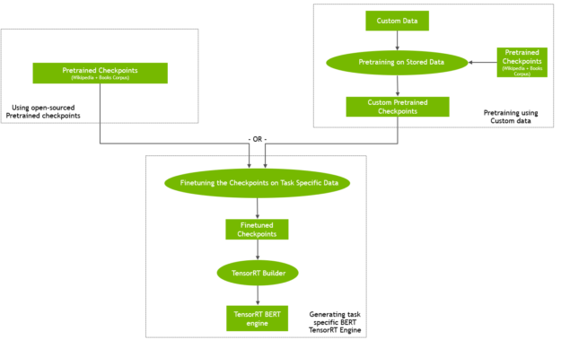
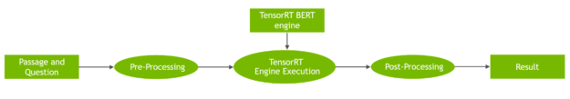
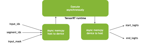
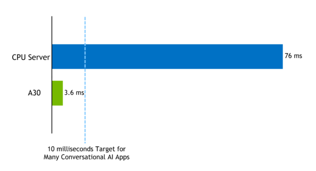
 The NVIDIA Merlin and KGMON team earned 1st place in the RecSys Challenge 2021 by effectively predicting the probability of user engagement within a dynamic environment and providing fair recommendations on a multi-million point dataset.
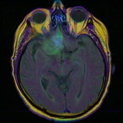


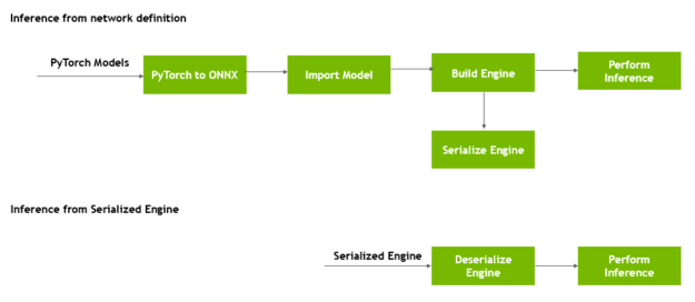
 ○ TensorRT is an SDK for high-performance deep learning inference and with TensorRT 8.0, you can import models trained using Quantization Aware Training (QAT) to run inference in INT8 precision without losing FP32 accuracy. QAT significantly reduces compute required and storage overhead for efficient inference.
 ) to an 8-bit representation (
 ), a scale-factor is used to map the floating-point tensor’s dynamic-range to [-128, 127]:
 is a function that applies some rounding-policy to round rational numbers to integers; and
  is a function that clips outliers that fall outside the [-128, 127] interval. TensorRT uses symmetric quantization to represent both activation data and model weights.
 ,
,  ]. Here,

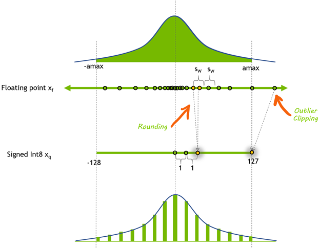
![x_{f} [-amax, amax]](https://s0.wp.com/latex.php?latex=x_%7Bf%7D+%5B-amax%2C+amax%5D&bg=ffffff&fg=000&s=0&c=20201002) is mapped through quantization to [-128, 127].
is mapped through quantization to [-128, 127].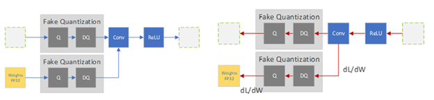
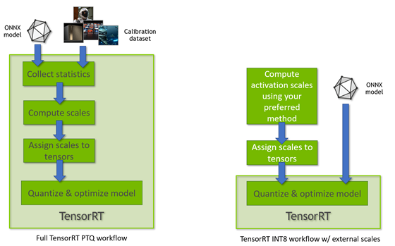
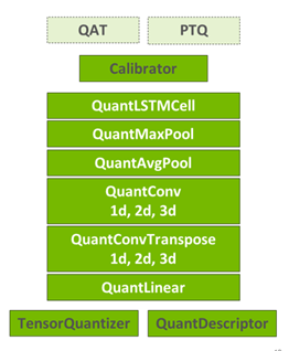
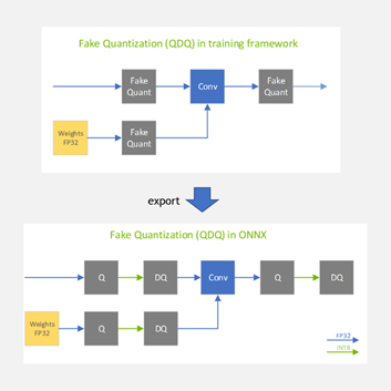
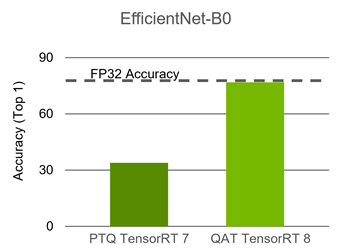
 This post is an introduction to deep learning-based recommender systems. It highlights the benefits of using neural networks and explains the different components. Neural network architectures are covered from the basic matrix factorization with deep learning up to session-based models.