submitted by /u/skj8
[visit reddit] [comments]
Categories
 DataBloom
submitted by /u/skj8
[visit reddit] [comments]

|
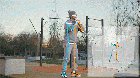
In order to better understand the human body for videos and images, pose detection is a critical step. Currently, many of us have tried 2D pose estimation with support from existing models. Tensorflow just launched their first 3D model in TF.js pose-detection API. An increasing interest from the TensorFlow.js community in 3D pose estimation has been seen, which opens up new design opportunities for applications such as fitness, medical and motion capture among many others. A great example of this is using 3D motion to drive a character animation on your browser. The community demo uses multiple models powered by MediaPipe and TensorFlow.js (namely FaceMesh, BlazePose, Hand Pose). It even works without app installation since a webpage is all you need to enjoy the experience. 5 Min Read | Live Demo | TensorFlow Blog submitted by /u/techsucker |
Hello, I’m training a segmentation model and it ends up freezing in the middle of training with no error. Running on a google cloud dedicated notebook with 2 GPUs (not COLAB), about 900 training images and it freezes in the middle of the ~30th epoch. For context it’s taking ~1.5 min per epoch with a batch size of 1 until it slows down and freezes. Wondering if this is a problem with google cloud cutting out or if I’m running out of room on my GPUs? I also included the resizing of the images and normalization of from 0-255 to 0-1 in the sequential model, can remove that if it is causing an issue but I doubt that’s the problem. Any advice very welcome, not finding much on SO or here. Cheers!
submitted by /u/quipkick
[visit reddit] [comments]
In March, a 28-car freight train derailment in Gibbons, Neb., forced Union Pacific to shut down three rail lines, delaying shipments nationwide for up to 48 hours and costing it millions as its rail network slowed down substantially. Fortunately, no one was injured. Duos Technologies, based in Jacksonville, Fla., says its NVIDIA GPU-accelerated AI railcar Read article >
The post Duos Technologies Uses AI-Powered Inspection to Help Railway Operators Stay on Track appeared first on The Official NVIDIA Blog.
 This NVIDIA Inception Spotlight features Resemble AI, a new generative voice technology startup able to create high-quality synthetic AI voices.
Deep learning is proving to be a powerful tool when it comes to high-quality synthetic speech development and customization. A Toronto-based startup, and NVIDIA Inception member, Resemble AI is upping the stakes with a new generative voice tool able to create high-quality synthetic AI Voices.
The technology can generate cross-lingual and naturally speaking voices in over 50 of the most popular languages, and with Resemble Fill, users can create programmatic audio and edit and replace words for audio clips.
The ability to build, deploy, and scale realistic AI voices stands to help a multitude of industries. The wide-ranging applications span from creating AI-generated text for advertisements, to interactive voice response systems, to video game development.
Since July 2020, the Resemble AI team has worked closely with the conversational AI team at NVIDIA to integrate the NVIDIA Riva multimodal conversational AI SDK into their speech pipeline. According to Resemble AI Founder and CEO, Zohaib Ahmed, the experience gave them unique insights into the entire conversational AI pipeline.
“The NVIDIA Inception Program has been helpful with providing key insights into the conversational AI space, as well as technical support on recommending GPU compute for every workload that we have as a product,” Ahmed said.
For training their speech models and inference, the team is using Amazon Elastic Kubernetes service (Amazon EKS) with clusters of NVIDIA T4 GPUs. They then use the NVIDIA Triton Inference Server to deploy their trained AI models at scale in production.
A recent demo of Resemble AI synthetic speech integrated with NVIDIA Omniverse Audio2Face showcases how the combined technology can create expressive facial animations and voices from a single audio source.
“Audio2Face is a good example of a powerful tool that can be combined easily with generative AI speech to produce results in seconds, which otherwise would take days,” Ahmed said.
The company has grown to host over 150,000 users, building over 60,000 voices. To date, Resemble AI has over 240 paying customers in various industries including telecommunication, finance, contact centers, education, gaming, and media and entertainment.
Do you have a startup? Join NVIDIA Inception’s global network of over 8,500 startups.
On June 2nd, 2021, Major League Baseball in the United States celebrated Lou Gehrig Day, commemorating both the day in 1925 that Lou Gehrig became the Yankees’ starting first baseman, and the day in 1941 that he passed away from amyotrophic lateral sclerosis (ALS, also known as Lou Gehrig’s disease) at the age of 37. ALS is a progressive neurodegenerative disease that affects motor neurons, which connect the brain with the muscles throughout the body, and govern muscle control and voluntary movements. When voluntary muscle control is affected, people may lose their ability to speak, eat, move and breathe.
In honor of Lou Gehrig, former NFL player and ALS advocate Steve Gleason, who lost his ability to speak due to ALS, recited Gehrig’s famous “Luckiest Man” speech at the June 2nd event using a recreation of his voice generated by a machine learning (ML) model. Gleason’s voice recreation was developed in collaboration with Google’s Project Euphonia, which aims to empower people who have impaired speaking ability due to ALS to better communicate using their own voices.
| Steve Gleason, who lost his voice to ALS, worked with Google’s Project Euphonia to generate a speech in his own voice in honor of Lou Gehrig. A portion of Gleason’s speech was broadcast in ballparks across the country during the 4th inning on June 2nd, 2021. |
Today we describe PnG NAT, the model adopted by Project Euphonia to recreate Steve Gleason’s voice. PnG NAT is a new text-to-speech synthesis (TTS) model that merges two state-of-the-art technologies, PnG BERT and Non-Attentive Tacotron (NAT), into a single model. It demonstrates significantly better quality and fluency than previous technologies, and represents a promising approach that can be extended to a wider array of users.
Recreating a Voice
Non-Attentive Tacotron (NAT) is the successor to Tacotron 2, a sequence-to-sequence neural TTS model proposed in 2017. Tacotron 2 used an attention module to connect the input text sequence and the output speech spectrogram frame sequence, so that the model knows which part of the text to pay attention to when generating each time step of the synthesized speech spectrogram. Tacotron 2 was the first TTS model that was able to synthesize speech that sounds as natural as a person speaking. However, with extensive experimentation we discovered that there is a small probability that the model can suffer from robustness issues — such as babbling, repeating, or skipping part of the text — due to the inherent flexibility of the attention mechanism.
NAT improves upon Tacotron 2 by replacing the attention module with a duration-based upsampler, which predicts a duration for each input phoneme and upsamples the encoded phoneme representation so that the output length corresponds to the length of the predicted speech spectrogram. Such a change both resolves the robustness issue, and improves the naturalness of the synthesized speech. This approach also enables precise control of the speech duration for each phoneme of the input text while still maintaining highly natural synthesis quality. Because recordings of people with ALS often exhibit disfluent speech, this ability to exert per-phoneme control is key for achieving the fluency of the recreated voice.
 |
| Non-Attentive Tacotron (NAT) model. |
While NAT addresses the robustness issue and enables precise duration control in neural TTS, we build upon it to further improve the natural language understanding of the TTS input. For this, we apply PnG BERT, which uses an approach similar to BERT, but is specifically designed for TTS. It is pre-trained with self-supervision on both the phoneme representation and the grapheme representation of the same content from a large text corpus, and then is used as the encoder of the TTS model. This results in a significant improvement of the prosody and pronunciation of the synthesized speech, especially in difficult cases.
Take, for example, the following audio, which was synthesized from a regular NAT model that takes only phonemes as input:
In comparison, the audio synthesized from PnG NAT on the same input text includes an additional pause that makes the meaning more clear.
The input text to both models is, “To cancel the payment, press one; or to continue, two.” Notice the different pause lengths before the ending “two” in the two versions. The word “two” in the version output by the regular NAT model could be confused for “too”. Because “too” and “two” have identical pronunciation (and thus the same phoneme representation), the regular NAT model does not understand which of the two is appropriate, and assumes it to be the word that more frequently follows a comma, “too”. In contrast, the PnG NAT model can more easily tell the difference, because it takes graphemes in addition to phonemes as input, and thus makes more appropriate pause.
The PnG NAT model integrates the pre-trained PnG BERT model as the encoder to the NAT model. The hidden representations output from the encoder are used by NAT to predict the duration of each phoneme, and are then upsampled to match the length of the audio spectrogram, as outlined above. In the final step, a non-attentive decoder converts the upsampled hidden representations into audio speech spectrograms, which are finally converted into audio waveforms by a neural vocoder.
 |
| PnG BERT and the pre-training objectives. Yellow boxes represent phonemes, and pink boxes represent graphemes. |
 |
| PnG NAT: PnG BERT replaces the original encoder in the NAT model. The random masking for the Masked Language Model (MLM) pre-training is removed. |
To recreate Steve Gleason’s voice, we first trained a PnG NAT model with recordings from 31 professional speakers, and then fine-tuned it with 30 minutes of Gleason’s recordings. Because these latter recordings were made after he was diagnosed with ALS, they exhibit signs of slurring. The fine tuned model was able to synthesize speech that sounds very similar to these recordings. However, because the symptoms of ALS were already present in Gleason’s speech, they exhibited some similar disfluencies.
To mitigate this, we leveraged the phoneme duration control of NAT as well as the model trained with professional speakers. We first predicted the durations of each phoneme for both a professional speaker and for Gleason, and then used the geometric mean of the two durations for each phoneme to guide the NAT output. As a result, the model is able to speak in Gleason’s voice, but more fluently than in the original recordings.
Here is the full version of the synthesized Lou Gehrig speech in Gleason’s voice:
<!– As a comparison, following is one of Gleason’s recordings that was used to train the model:
–>
Besides recreating voices for people with ALS, PnG NAT is also powering voices for a variety of customers through Google Cloud Custom Voice.
Project Euphonia
Of the millions of people around the world who have neurologic conditions that may impact their speech, such as ALS, cerebral palsy or Down syndrome, many may find it difficult to be understood, which can make face-to-face communication challenging. Using voice-activated technologies can be frustrating too, as they don’t always work reliably. Project Euphonia is a Google Research initiative focused on helping people with impaired speech be better understood. The team is researching ways to improve speech recognition for individuals with speech impairments (see recent blog post and segment in TODAY show), as well as customized text-to-speech technology (see Age of AI documentary featuring former NFL player Tim Shaw).
Acknowledgements
Many people across Google Research, Google Cloud and Consumer Apps, and Google Accessibility teams contributed to this project and the event, including Michael Brenner, Bob MacDonald, Heiga Zen, Yu Zhang, Jonathan Shen, Isaac Elias, Yonghui Wu, Anne Keck, Danielle Notaro, Kevin Hogan, Zack Kaplan, KR Liu, Kyndra Price, Zoe Ortiz.

Hi I recently created a small image binary classification project and was wondering how I could deploy it to the web.
I’ve been able to convert the model to .json but I don’t know what to do next.
I’m trying to make it so that the user can upload an image or provide a image link and then the model preprocesses the image to the correct size and then uses the model to predict.
Anyone know how to do this?
submitted by /u/Sad_Combination9971
[visit reddit] [comments]
I’m currently learning HTML, CSS and JavaScript (still at an introductory level) and I am looking to explore machine learning via tensorflow.js. I was wondering if the following web app idea could be built using tensorflow.js or if anyone has any recommendations for frameworks that I could learn to achieve something like this?
Idea: – similar to Akinator (guessing a celebrity based off asking questions) but only for sports players – first ask the user to input as much information as possible into a text area box – not sure if this is possible, but can tensorflow.js scan for key words that has been inputted in the text area? – then if the web app needs to ask more questions (to come to a guess), they will ask some more (and use information from the text area + from different userInput to guide the questions asked) – then output a guess! – then this info can get stored to improve guessing for the next user
For example: – user inputs “Basketball player at Los Angeles laker. Tall. Number 23” into text area – AI can then ask “was your player previously at Miami Heat.” Etc etc – AI outputs guess: Lebron James – AI stores this information for next user
Very new to computer science so I’m not sure what avenue I would take to create something like this. But any suggestions regarding how I should approach this/what I should learn would be appreciated!
submitted by /u/cookie_monster2017
[visit reddit] [comments]
When tensorflow has tf.image.* for image augmentation, why should we use ImageDataGenerator?
I feel, tf.image.* is easier, But many tutorials, ImageDataGenerator has been used.
Please someone clarify this.
Thanks
submitted by /u/mahesh2150
[visit reddit] [comments]
Hey, I have trained multi out model in colab the model branch one will classify an image using passion loss the other branch will segment using binary crossentropy loss and using dicecoef as accuracy , when trained on colab the model gives good result accuracy:99,dicecoef:90
however when trained on my local machine one of two usually accurcuy randomly go to zero , nothing has changed used same code , same data only difference is I used tensorflow 2.5 while on colab it was 2.6.
I appoliges for the dirty codeing.
import os
os.environ[‘TF_CPP_MIN_LOG_LEVEL’] = ‘3’ # or any {‘0’, ‘1’, ‘2’}
import tensorflow as tf
import random
import numpy as np
import matplotlib.pyplot as plt
from tqdm import tqdm
from skimage.io import imread , imshow
from skimage.transform import resize
# example of pixel normalization
from numpy import asarray
# load image
import shutil
#import cv2 as cv
import tensorflow.keras.backend as K
from tensorflow.keras.losses import binary_crossentropy
beta = 0.25
alpha = 0.25
gamma = 2
epsilon = 1e-5
smooth = 1
class Semantic_loss_functions(object):
def __init__(self):
print (“semantic loss functions initialized”)
def dice_coef(self, y_true, y_pred):
y_true_f = K.flatten(y_true)
y_pred_f = K.flatten(y_pred)
intersection = K.sum(y_true_f * y_pred_f)
return (2. * intersection + K.epsilon()) / (
K.sum(y_true_f) + K.sum(y_pred_f) + K.epsilon())
def sensitivity(self, y_true, y_pred):
true_positives = K.sum(K.round(K.clip(y_true * y_pred, 0, 1)))
possible_positives = K.sum(K.round(K.clip(y_true, 0, 1)))
return true_positives / (possible_positives + K.epsilon())
def specificity(self, y_true, y_pred):
true_negatives = K.sum(
K.round(K.clip((1 – y_true) * (1 – y_pred), 0, 1)))
possible_negatives = K.sum(K.round(K.clip(1 – y_true, 0, 1)))
return true_negatives / (possible_negatives + K.epsilon())
def convert_to_logits(self, y_pred):
y_pred = tf.clip_by_value(y_pred, tf.keras.backend.epsilon(),
1 – tf.keras.backend.epsilon())
return tf.math.log(y_pred / (1 – y_pred))
def weighted_cross_entropyloss(self, y_true, y_pred):
y_pred = self.convert_to_logits(y_pred)
pos_weight = beta / (1 – beta)
loss = tf.nn.weighted_cross_entropy_with_logits(logits=y_pred,
targets=y_true,
pos_weight=pos_weight)
return tf.reduce_mean(loss)
def focal_loss_with_logits(self, logits, targets, alpha, gamma, y_pred):
weight_a = alpha * (1 – y_pred) ** gamma * targets
weight_b = (1 – alpha) * y_pred ** gamma * (1 – targets)
return (tf.math.log1p(tf.exp(-tf.abs(logits))) + tf.nn.relu(
-logits)) * (weight_a + weight_b) + logits * weight_b
def focal_loss(self, y_true, y_pred):
y_pred = tf.clip_by_value(y_pred, tf.keras.backend.epsilon(),
1 – tf.keras.backend.epsilon())
logits = tf.math.log(y_pred / (1 – y_pred))
loss = self.focal_loss_with_logits(logits=logits, targets=y_true,
alpha=alpha, gamma=gamma, y_pred=y_pred)
return tf.reduce_mean(loss)
def depth_softmax(self, matrix):
sigmoid = lambda x: 1 / (1 + K.exp(-x))
sigmoided_matrix = sigmoid(matrix)
softmax_matrix = sigmoided_matrix / K.sum(sigmoided_matrix, axis=0)
return softmax_matrix
def generalized_dice_coefficient(self, y_true, y_pred):
smooth = 1.
y_true_f = K.flatten(y_true)
y_pred_f = K.flatten(y_pred)
intersection = K.sum(y_true_f * y_pred_f)
score = (2. * intersection + smooth) / (
K.sum(y_true_f) + K.sum(y_pred_f) + smooth)
return score
def dice_loss(self, y_true, y_pred):
loss = 1 – self.generalized_dice_coefficient(y_true, y_pred)
return loss
def bce_dice_loss(self, y_true, y_pred):
loss = binary_crossentropy(y_true, y_pred) +
self.dice_loss(y_true, y_pred)
return loss / 2.0
def confusion(self, y_true, y_pred):
smooth = 1
y_pred_pos = K.clip(y_pred, 0, 1)
y_pred_neg = 1 – y_pred_pos
y_pos = K.clip(y_true, 0, 1)
y_neg = 1 – y_pos
tp = K.sum(y_pos * y_pred_pos)
fp = K.sum(y_neg * y_pred_pos)
fn = K.sum(y_pos * y_pred_neg)
prec = (tp + smooth) / (tp + fp + smooth)
recall = (tp + smooth) / (tp + fn + smooth)
return prec, recall
def true_positive(self, y_true, y_pred):
smooth = 1
y_pred_pos = K.round(K.clip(y_pred, 0, 1))
y_pos = K.round(K.clip(y_true, 0, 1))
tp = (K.sum(y_pos * y_pred_pos) + smooth) / (K.sum(y_pos) + smooth)
return tp
def true_negative(self, y_true, y_pred):
smooth = 1
y_pred_pos = K.round(K.clip(y_pred, 0, 1))
y_pred_neg = 1 – y_pred_pos
y_pos = K.round(K.clip(y_true, 0, 1))
y_neg = 1 – y_pos
tn = (K.sum(y_neg * y_pred_neg) + smooth) / (K.sum(y_neg) + smooth)
return tn
def tversky_index(self, y_true, y_pred):
y_true_pos = K.flatten(y_true)
y_pred_pos = K.flatten(y_pred)
true_pos = K.sum(y_true_pos * y_pred_pos)
false_neg = K.sum(y_true_pos * (1 – y_pred_pos))
false_pos = K.sum((1 – y_true_pos) * y_pred_pos)
alpha = 0.7
return (true_pos + smooth) / (true_pos + alpha * false_neg + (
1 – alpha) * false_pos + smooth)
def tversky_loss(self, y_true, y_pred):
return 1 – self.tversky_index(y_true, y_pred)
def focal_tversky(self, y_true, y_pred):
pt_1 = self.tversky_index(y_true, y_pred)
gamma = 0.75
return K.pow((1 – pt_1), gamma)
def log_cosh_dice_loss(self, y_true, y_pred):
x = self.dice_loss(y_true, y_pred)
return tf.math.log((tf.exp(x) + tf.exp(-x)) / 2.0)
########
n_filters=50
epochs=50
batch_size=6
Img_wedth =128
Img_height = 128
Img_channels = 1
#####################################
import h5py
paths=os.listdir(‘C:/Users/ASUS/Desktop/imageData/’)
## save images in arrays ##
X_train = np.zeros((len(paths) , Img_height , Img_wedth , Img_channels) , dtype = np.float32)
y_train = np.zeros((len(paths) , Img_height , Img_wedth , Img_channels ) , dtype = np.float32)
y_train_label=[]
#####################################
for n, id_ in tqdm(enumerate(paths) , total = len(paths)) :
ttt=[0,0,0]
path = ‘C:/Users/ASUS/Desktop/imageData/’+id_
#print(‘path.. ‘,path)
#print(‘id.. ‘,id_)
#img = imread(path + ‘/image/’ +id_ + ‘.png’) [: , : ]
img1=h5py.File(path,’r’)
# print(‘path.. ‘,path)
img=img1[‘cjdata’][‘image’]
img = resize(img , (Img_height , Img_wedth , Img_channels) , mode = ‘constant’ , preserve_range=True)
#print(img.shape)
# imshow(img,cmap=”gray”)
# plt.show()
img = asarray(img)
img = img.astype(‘float32’)
# normalize to the range 0-1
img = tf.image.per_image_standardization(img)
# print(img[55][55])
#print(img.shape)
X_train[n] = img
# print(‘path.. ‘,path)
mask=img1[‘cjdata’][‘tumorMask’]
mask = asarray(mask)
mask = mask.astype(‘float32’)
#_,mask=cv.threshold(mask, 0.01, 1, 0 )
mask = resize(mask , (Img_height , Img_wedth , Img_channels) , mode = ‘constant’ , preserve_range=True)
#print(img.shape)
# imshow(img,cmap=”gray”)
# plt.show()
# normalize to the range 0-1
ttt[int(img1[‘cjdata’][‘label’][0][0])-1]=img1[‘cjdata’][‘label’][0][0]
y_train_label.append(ttt)
y_train[n] = mask
# print(Mask_[55][55])
# Mask_ = np.expand_dims(resize(Mask_ , (Img_height , Img_wedth) , mode = ‘constant’ ,
# preserve_range = True) , axis = -1)
# Mask = np.maximum(Mask , Mask_ )
# Mask = np.zeros((Img_height , Img_wedth , 1) , dtype = np.bool)
y_train_label=np.array(y_train_label)
paths_test=os.listdir(‘C:/Users/ASUS/Desktop/test’)[10:20]
X_test = np.zeros((len(paths_test) , Img_height , Img_wedth , Img_channels ) , dtype = np.float32)
y_test = np.zeros((len(paths_test) , Img_height , Img_wedth , Img_channels ) , dtype = np.float32)
y_test_label= []
print(‘resizing test images’)
for n, id_ in tqdm(enumerate(paths_test) , total = len(paths_test)) :
path = ‘C:/Users/ASUS/Desktop/test/’+id_
ttt1=[0,0,0]
img1=h5py.File(path,’r’)
# print(‘path.. ‘,path)
img=img1[‘cjdata’][‘image’]
img = resize(img , (Img_height , Img_wedth , Img_channels) , mode = ‘constant’ , preserve_range=True)
#print(img.shape)
# imshow(img,cmap=”gray”)
# plt.show()
img = asarray(img)
img = img.astype(‘float32’)
img = tf.image.per_image_standardization(img)
# normalize to the range 0-1
X_test[n]=img
mask=h5py.File(path,’r’)
# print(‘path.. ‘,path)
mask1=mask[‘cjdata’][‘tumorMask’]
mask1 = asarray(mask1)
mask1 = mask1.astype(‘float32’)
# _,mask1=cv.threshold(mask1, 0.01, 1, 0 )
mask1 = resize(mask1 , (Img_height , Img_wedth , Img_channels) , mode = ‘constant’ , preserve_range=True)
#print(img.shape)
# imshow(img,cmap=”gray”)
# plt.show()
# normalize to the range 0-1
ttt1[int(img1[‘cjdata’][‘label’][0][0])-1]=img1[‘cjdata’][‘label’][0][0]
y_test_label.append(ttt1)
y_test[n]=mask1
#print(‘imagetestid..’,n,’imagetestname’,id_)
#imshow(img)
#plt.show()
#image_x = random.randint(0 , len(Train_ids))
#imshow(X_train[image_x])
#plt.show()
#imshow(np.squeeze( y_train[image_x]))
#plt.show()
## U-net Moudel
inputs = tf.keras.Input((Img_wedth , Img_height , Img_channels ))
c1 = tf.keras.layers.Conv2D(n_filters*1 , (3,3) , activation=’relu’
, kernel_initializer=’he_normal’ , padding=’same’)(inputs)
c1 = tf.keras.layers.Dropout(0.1 )(c1)
p1 = tf.keras.layers.MaxPooling2D((2,2 ))(c1)
print (‘Done_c1’)
c2 = tf.keras.layers.Conv2D(n_filters*2 , (3,3) , activation=’relu’
, kernel_initializer=’he_normal’ , padding=’same’)(p1)
c2 = tf.keras.layers.Dropout(0.1 )(c2)
p2 = tf.keras.layers.MaxPooling2D((2,2 ))(c2)
print (‘Done_c2’)
c3 = tf.keras.layers.Conv2D(n_filters*4 , (3,3) , activation=’relu’
, kernel_initializer=’he_normal’ , padding=’same’)(p2)
c3 = tf.keras.layers.Dropout(0.2 )(c3)
p3 = tf.keras.layers.MaxPooling2D((2,2 ))(c3)
print (‘Done_c3’)
c4 = tf.keras.layers.Conv2D(n_filters*8 , (3,3) , activation=’relu’
, kernel_initializer=’he_normal’ , padding=’same’)(p3)
c4 = tf.keras.layers.Dropout(0.2 )(c4)
p4 = tf.keras.layers.MaxPooling2D(pool_size=((2,2 )))(c4)
print (‘Done_c4’)
c5 = tf.keras.layers.Conv2D(n_filters*16 , (3,3) , activation=’relu’
, kernel_initializer=’he_normal’ , padding=’same’)(p4)
c5 = tf.keras.layers.Dropout(0.3 )(c5)
c5 = tf.keras.layers.Conv2D(n_filters*16, (3,3) , activation=’relu’
, kernel_initializer=’he_normal’ , padding=’same’)(c5)
print (‘Done_c5’)
F1=tf.keras.layers.Flatten()(c5)
D1=tf.keras.layers.Dense(32,activation=’relu’)(F1)
D2=tf.keras.layers.Dense(3,activation=’softmax’,name=’clas’)(D1)
u6 = tf.keras.layers.Conv2DTranspose(n_filters*8 , (2,2) , strides=(2,2) , padding=’same’)(c5)
print (‘Done_c61’)
u6 = tf.keras.layers.Concatenate(axis=-1)([u6 , c4])
print (‘Done_c62’)
c6 = tf.keras.layers.Conv2D(n_filters*8 ,(3,3) , activation=’relu’
, kernel_initializer=’he_normal’ , padding=’same’)(u6)
print (‘Done_c63’)
c6 = tf.keras.layers.Dropout(0.2 )(c6)
c6 = tf.keras.layers.Conv2D(n_filters*8, (3,3) , activation=’relu’
, kernel_initializer=’he_normal’ , padding=’same’)(c6)
print (‘Done_c6’)
u7 = tf.keras.layers.Conv2DTranspose(n_filters*4 , (2,2) , strides=(2,2) , padding=’same’)(c6)
u7 = tf.keras.layers.Concatenate(axis=-1)([u7 , c3])
c7 = tf.keras.layers.Conv2D(n_filters*4 , (3,3) , activation=’relu’
, kernel_initializer=’he_normal’ , padding=’same’)(u7)
c7 = tf.keras.layers.Dropout(0.2 )(c7)
c7 = tf.keras.layers.Conv2D(n_filters*4 , (3,3) , activation=’relu’
, kernel_initializer=’he_normal’ , padding=’same’)(c7)
print (‘Done_c7’)
u8 = tf.keras.layers.Conv2DTranspose(n_filters*2 , (2,2) , strides=(2,2) , padding=’same’)(c7)
u8 = tf.keras.layers.Concatenate(axis=-1)([u8 , c2])
c8 = tf.keras.layers.Conv2D(n_filters*2 , (3,3) , activation=’relu’
, kernel_initializer=’he_normal’ , padding=’same’)(u8)
c8 = tf.keras.layers.Dropout(0.2)(c8)
c8 = tf.keras.layers.Conv2D(n_filters*2 , (3,3) , activation=’relu’
, kernel_initializer=’he_normal’ , padding=’same’)(c8)
print (‘Done_c8’)
u9 = tf.keras.layers.Conv2DTranspose(n_filters*1 , (2,2) , strides=(2,2) , padding=’same’)(c8)
print (‘Done_c91’)
u9 = tf.keras.layers.Concatenate(axis=-1)([u9 , c1])
print (‘Done_c92’)
c9 = tf.keras.layers.Conv2D(n_filters*1 , (3,3) , activation=’relu’
, kernel_initializer=’he_normal’ , padding=’same’)(u9)
print (‘Done_c93’)
c9 = tf.keras.layers.Dropout(0.4)(c9)
print (‘Done_c94’)
c9 = tf.keras.layers.Conv2D(n_filters*1 , (3,3) , activation=’relu’
, kernel_initializer=’he_normal’ , padding=’same’)(c9)
print (‘Done_c9’)
outputs = tf.keras.layers.Conv2D(1 , (1,1) , activation=’sigmoid’,name=’seg’)(c9)
print (‘Done_out’)
model = tf.keras.Model(inputs=[inputs] , outputs=[outputs,D2])
print (‘Done_model1’)
def dice_coef1(y_true, y_pred, smooth=1):
print(y_true.shape,y_pred.shape)
intersection = K.sum((y_true )*( tf.round(y_pred)), axis=[1,2,3])
union = K.sum((y_true), axis=[1,2,3]) + K.sum((tf.round(y_pred)), axis=[1,2,3])
dice = K.mean((2. * intersection + smooth)/(union + smooth), axis=0)
return dice
loss={“seg”:binary_crossentropy,
“clas”:tf.keras.losses.poisson}
metricss={‘seg’:dice_coef1,
‘clas’:’Accuracy’}
opt=tf.keras.optimizers.Adam(clipvalue=1,clipnorm=1,lr=0.0001)
s = Semantic_loss_functions()
model.compile(optimizer=opt, loss=loss, metrics=metricss)
model.summary()
#############
# modelchecpoints
from tensorflow.keras import callbacks
results = model.fit(X_train , [y_train,y_train_label] ,shuffle=True, batch_size =batch_size, epochs=epochs )
submitted by /u/Ali99695
[visit reddit] [comments]