
 Machine Learning Frameworks Interoperability part 3 covers on the implementation of an end-to-end pipeline demonstrating the discussed techniques for optimal data transfer across data science frameworks.
Introduction
Efficient pipeline design is crucial for data scientists. When composing complex end-to-end workflows, you may choose from a wide variety of building blocks, each of them specialized for a dedicated task. Unfortunately, repeatedly converting between data formats is an error-prone and performance-degrading endeavor. Let’s change that!
In this blog series, we discuss different aspects of efficient framework interoperability:
- In the first post, we discussed pros and cons of distinct memory layouts as well as memory pools for asynchronous memory allocation to enable zero-copy functionality.
- In the second post, we highlighted bottlenecks occurring during data loading/transfers and how to mitigate them using Remote Direct Memory Access (RDMA) technology.
- In this post, we dive into the implementation of an end-to-end pipeline demonstrating the discussed techniques for optimal data transfer across data science frameworks.
To learn more on framework interoperability, check out our presentation at NVIDIA’s GTC 2021 Conference.
Let’s dive into the implementation details of a fully functional pipeline for:
- Parsing of 20 hours of continuously measured electrocardiograms (ECGs) from plain CSV files.
- Unsupervised segmentation of bespoke ECG stream into individual heart beats using traditional signal processing techniques.
- Subsequent training of a variational autoencoder (VAE) for outlier detection.
- Final visualization of the results.
For each of the previous steps, a different data science library is used, so making efficient data conversion a crucial task. Most importantly, you should avoid costly CPU roundtrips when copying data from one GPU-based framework to another.
Zero-Copy in Action: End-to-End pipeline
Enough talk! Let’s see framework interoperability in action. In the following, we will discuss the end-to-end pipeline step by step. If you are an impatient person, you can directly download the full Jupyter notebook here. The source code can be executed from within a recent RAPIDS docker container.
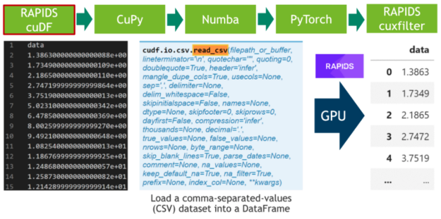
Step 1: Data loading
In the first step, we download 20 hours of electrocardiograms as a CSV file and write it to disk (see Cell 1). After, we parse the 500 MB of scalar values from the CSV file and transfer them directly to the GPU using RAPIDS’ blazing fast CSV reader (see Cell 2). Now, the data resides on the GPU and will stay there until the very end. Next, we plot the whole time series consisting of 20 million scalar data points using the cuxfilter (ku-cross-filter) framework (see Cell 3).
Step 2: Data segmentation
In the next step, we segment the 20 hours ECG into individual heartbeats using traditional signal processing techniques. We achieve that by convolving the ECG stream with the second derivative of a Gaussian distribution, also known as Ricker wavelet, in order to isolate the corresponding frequency band of the initial peak in a prototypical heartbeat. Both the sampling of the wavelet as well as the FFT-based convolution are facilitated using CuPy, a CUDA-accelerated library for dense linear algebra and array operations. As a direct result, the RAPIDS cuDF dataframe storing the ECG data has to be converted to a CuPy array using DLPack as a zero-copy mechanism.
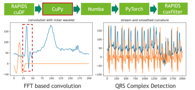
The feature response (result) of the convolution measures the presence of a fixed frequency content for each position in the stream. Note that we have chosen the wavelet in a way so that local maxima correspond to the initial peak of a heartbeat.
Step 3: Local maxima detection
In the next step, we map these extremal points to a binary gate using a 1D variant of non-maximum suppression (NMS). NMS determines for every position in the stream if the corresponding value is the maximum in a predefined window (neighborhood). A CUDA implementation of this embarrassingly parallel problem is straightforward. In our example, we use the just-in-time compiler Numba to allow for seamless Python integration. Both Numba and Cupy implement the CUDA array interface as a zero-copy mechanism and thus the explicit cast from CuPy arrays to Numba device arrays can be fully avoided.
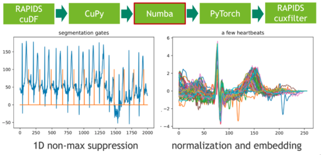
The length of each heartbeat is determined by computing the adjacent difference (finite step derivative) of the gate positions. We facilitate this by filtering the index domain with the predicate gate==1 followed by a call to cupy.diff(). The resulting histogram depicts the length distribution.
Step 4: Candidate pruning and embedding
We intend to train a (convolutional) Variational Autoencoder (VAE) on the set of heartbeats using a fixed-length input matrix. The embedding of heartbeats in a vector of zeros can be realized with a CUDA kernel. Here, we again use Numba for both candidate pruning and embedding.
Step 5: Outliers detection
In this step, we train the VAE model on 75% of the data. DLPack is used again as the zero-copy mechanism to map the CuPy data matrix to a PyTorch tensor.
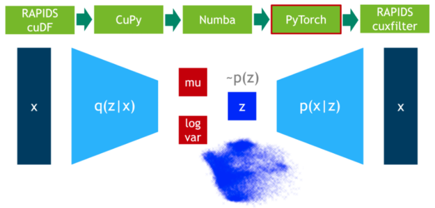
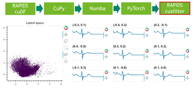
Step 6: Results visualization
In a final step, we visualize the latent space of the remaining 25% of the data.
Conclusion
A key takeaway from this and the preceding blog posts is that interoperability is crucial for the design of efficient data pipelines. Copy-and-converting data between different frameworks is an expensive and incredibly time-consuming task that adds zero value to data science pipelines. Data science workloads are becoming increasingly complex, and the interaction between multiple software libraries is common practice. DLPack and the CUDA Array Interface are the de facto data format standards that guarantee zero-copy data exchange among GPU-based frameworks.
Support for external memory managers is a nice-to-have feature to consider when appraising which software libraries your pipeline will use. For instance, if your task requires both DataFrame and array data manipulation, a great choice of libraries is RAPIDS cuDF + CuPy. They both benefit from GPU acceleration, support DLPack to exchange data with zero-copy, and share the same memory manager, RMM. Alternatively, RAPIDS cuDF + JAX would also be an excellent option. Nevertheless, the latter combination might require extra development efforts to leverage memory usage because of JAX’s lack of support for external memory allocators.
Data loading and data transfer bottlenecks are frequent when dealing with large datasets. NVIDIA GPUDirect technology comes to the rescue, supporting moving data into or out of the GPU memory without burdening the CPU and reducing to one the number of data copies needed when transferring data between GPUs on different nodes.