Categories
Misc

Simplifying Model Development and Building Models at Scale with PyTorch Lightning and NGC

PyTorch Lightning is a lightweight PyTorch wrapper for high-performance AI research. PyTorch code with Lightning enables seamless training on multiple-GPUs and uses best practices such as checkpointing, logging, sharding, and mixed precision. In this post, we walk you through building speech models with PyTorch Lightning on NVIDIA GPU-powered AWS instances managed by the Grid.ai platform.

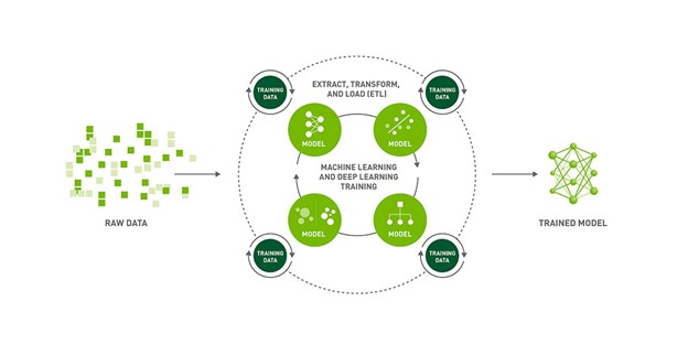
AI is driving the fourth Industrial Revolution with machines that can hear, see, understand, analyze, and then make smart decisions at superhuman levels. However, the effectiveness of AI depends on the quality of the underlying models. So, whether you’re an academic researcher or a data scientist, you want to quickly build models with a variety of parameters and identify the most effective ones for your solutions.

In this post, we walk you through building speech models with PyTorch Lightning on NVIDIA GPU-powered AWS instances.

PyTorch Lightning + Grid.ai: Build models faster, at scale

PyTorch Lightning is a lightweight PyTorch wrapper for high-performance AI research. Organizing PyTorch code with Lightning enables seamless training on multiple GPUs, TPUs, CPUs, and the use of difficult to implement best practices such as checkpointing, logging, sharding, and mixed precision. A PyTorch Lightning container and developer environment is available on the NGC catalog.

Grid enables you to scale training from your laptop to the cloud without having to modify your code. Running on cloud providers such as AWS, Grid supports Lightning as well as all the classic machine learning frameworks such as Sci Kit, TensorFlow, Keras, PyTorch and more. With Grid, you can scale the training of models from the NGC catalog.

NGC: The hub for GPU-optimized AI software

The NGC catalog is the hub for GPU-optimized software including AI/ML containers, pretrained models, and SDKs that can be easily deployed across on-premises, cloud, edge, and hybrid environments. NGC offers NVIDIA TAO Toolkit that enables retraining models with custom data and NVIDIA Triton Inference Server to run predictions on CPU and GPU-powered systems.

The rest of this post walks you through how to leverage models from the NGC catalog and the NVIDIA NeMo framework to train an automatic speech recognition (ASR) model with PyTorch Lightning using the following tutorial based on the ASR with NeMo tutorial.

Raw data is trained, evaluated, iterated, and retrained for highly accurate results and performant models.
Figure 1. AI model training process

Training NGC models with Grid sessions, PyTorch Lightning, and NVIDIA NeMo

ASR is the task of transcribing spoken language to text and is a critical component of Speech to Text systems. When training ASR models, your goal is to generate text from a given audio input that minimizes the word error rate (WER) metric on human transcribed speech. The NGC catalog contains state-of-the-art pretrained models for ASR.

In the remainder of this post, we show you how to use Grid sessions, NVIDIA NeMo, and PyTorch Lightning to fine-tune these models on the AN4 dataset.

The AN4 dataset, also known as the Alphanumeric dataset, was collected and published by Carnegie Mellon University. It consists of recordings of people spelling out addresses, names, telephone numbers, and so on, one letter or number at a time, as well as their corresponding transcripts.

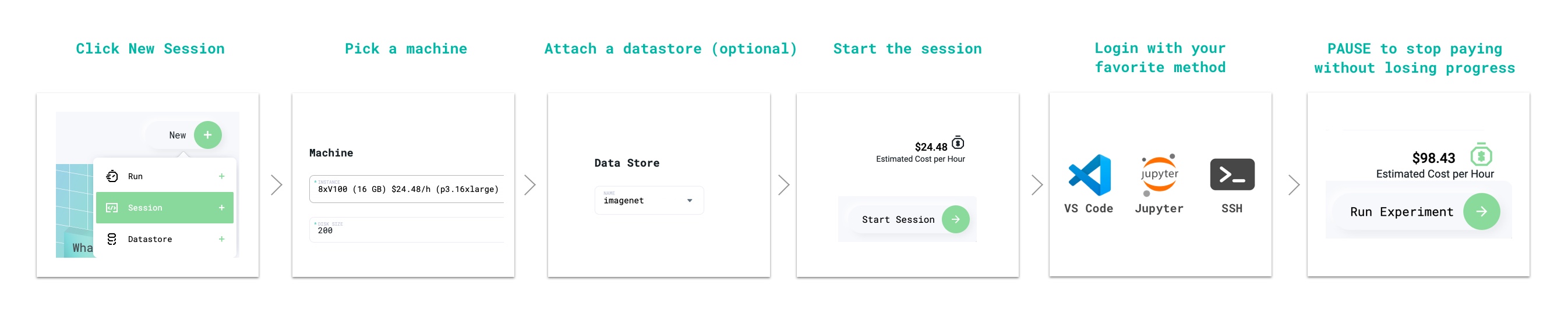
Step 1: Create a Grid session optimized for Lightning and pretrained NGC models

Grid sessions run on the same hardware that you need to scale while providing you with preconfigured environments to iterate the research phase of the machine learning process faster than before. Sessions are linked to GitHub, loaded with JupyterHub, and can be accessed through SSH and your IDE of choice without having to do any setup yourself.

With sessions, you pay only for the compute that you need to get a baseline operational, and then you can scale your work to the cloud with Grid runs. Grid sessions are optimized for PyTorch Lightning and models hosted on the NGC catalog. They even provide specialized Spot pricing.

For an in-depth walkthrough, see the Grid Session tour (requires a Grid.ai account).

Step-by-step process to create a Grid session optimized for PyTorch Lightning: Choose New Session, Pick a machine, attach a datastore, start the session, log in, and pause to stop paying without losing progress.
Figure 2. Workflow to create a Grid session

Step 2: Clone the ASR demo repo and open the tutorial notebook

Now that you have a developer environment optimized for PyTorch Lightning, the next step is to clone the NGC-Lightning-Grid-Workshop repo.

You can do this directly from a terminal in your Grid Session with the following command:

git clone https://github.com/aribornstein/NGC-Lightning-Grid-Workshop.git

After you’ve cloned the repo, you can open up the notebook to use to fine-tune the NGC hosted model with NeMo and PyTorch Lightning.

Step 3: Install NeMo ASR dependencies

First, install all the session dependencies. Run tools such as PyTorch Lightning and NeMo and process the AN4 dataset to do this. Run the first cell in the tutorial notebook, which runs the following bash commands to install the dependencies.

## Install dependencies
!pip install wget
!sudo apt-get install sox libsndfile1 ffmpeg -y
!pip install unidecode
!pip install matplotlib>=3.3.2
## Install NeMo
BRANCH = 'main'
!python -m pip install --user git+https://github.com/NVIDIA/NeMo.git@$BRANCH#egg=nemo_toolkit[all]
## Grab the config we'll use in this example
!mkdir configs
!wget -P configs/ https://raw.githubusercontent.com/NVIDIA/NeMo/$BRANCH/examples/asr/conf/config.yaml

Step 4: Convert and visualize the AN4 dataset

The AN4 dataset comes in raw Sof audio files, but most models process on mel spectrograms.  Convert the Sof files to the Wav format so that you can use NeMo audio processing.

import librosa
import IPython.display as ipd
import glob
import os
import subprocess
import tarfile
import wget

# Download the dataset. This will take a few moments...
print("******")
if not os.path.exists(data_dir + '/an4_sphere.tar.gz'):
    an4_url = 'http://www.speech.cs.cmu.edu/databases/an4/an4_sphere.tar.gz'
    an4_path = wget.download(an4_url, data_dir)
    print(f"Dataset downloaded at: {an4_path}")
else:
    print("Tarfile already exists.")
    an4_path = data_dir + '/an4_sphere.tar.gz'

if not os.path.exists(data_dir + '/an4/'):
    # Untar and convert .sph to .wav (using sox)
    tar = tarfile.open(an4_path)
    tar.extractall(path=data_dir)

    print("Converting .sph to .wav...")
    sph_list = glob.glob(data_dir + '/an4/**/*.sph', recursive=True)
    for sph_path in sph_list:
        wav_path = sph_path[:-4] + '.wav'
        cmd = ["sox", sph_path, wav_path]
        subprocess.run(cmd)
print("Finished conversion.n******")
# Load and listen to the audio file
example_file = data_dir + '/an4/wav/an4_clstk/mgah/cen2-mgah-b.wav'
audio, sample_rate = librosa.load(example_file)
ipd.Audio(example_file, rate=sample_rate)

You can then visualize the audio example as images of the audio waveform. Figure 3 shows the activity in the waveform that corresponds to each letter in the audio, as your speaker here enunciates quite clearly!

Example of five letters in audio wave form.
Figure 3. Audio waveform of the sample example

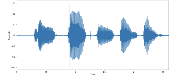
Each spoken letter has a different “shape.” It’s interesting to note that the last two blobs look relatively similar, which is expected because they are both the letter N.

Spectrograms

Modeling audio is easier in the context of frequencies of sound over time. You can get a better representation than this raw sequence of 57,330 values. A spectrogram is a good way of visualizing how the strengths of various frequencies in the audio vary over time. It is obtained by breaking up the signal into smaller, usually overlapping chunks, and performing a short-time Fourier transform (STFT) on each.

Figure 4 shows what the spectrogram of the sample looks like.

Waveform diagram of audio spectrogram where each letter is being pronounced
Figure 4. Audio spectrogram of the sample example

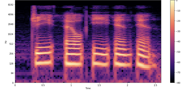
As in the earlier waveform, you see each letter being pronounced. How do you interpret these shapes and colors? Just as in the earlier waveform plot, you see time passing on the x-axis (all 2.6s of audio). However, now the y-axis represents different frequencies (on a log scale), and the color on the plot shows the strength of a frequency at a particular point in time.
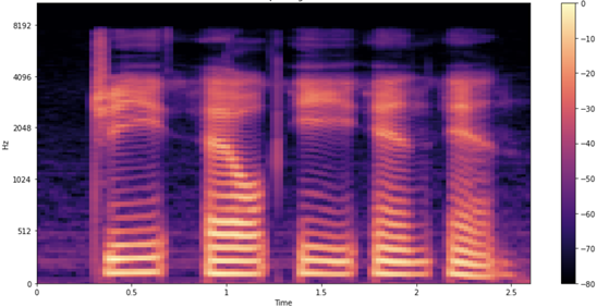
Mel spectrograms

You’re still not done, as you can make one more potentially useful tweak by visualizing the data using the mel spectrogram. Change the frequency scale from linear (or logarithmic) to the mel scale, which better represents the pitches that are perceivable to the human ear. Mel spectrograms are intuitively useful for ASR. Because you are processing and transcribing human speech, mel spectrograms reduce background noise that can affect the model.

Example of Mel spectrogram useful for ASR
Figure 5. Mel spectrogram of the sample example

Step 5: Load and inference a pretrained QuartzNet model from NGC

Now that you’ve loaded and properly understood the AN4 dataset, look at how to use NGC to load an ASR model to be fine-tuned with PyTorch Lightning. NeMo’s ASR collection comes with many building blocks and even complete models that you can use for training and evaluation. Moreover, several models come with pretrained weights.

To model the data for this post, you use a Jasper architecture called QuartzNet from the NGC Model Hub. Jasper architecture consists of repeated block structures that uses 1D convolutions to model spectrogram data (Figure 6).

Jasper/Quartz model that displays how Jasper architecture uses 1D convolutions to model spectrogram data
Figure 6. Jasper/QuartzNet model

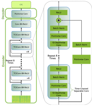
QuartzNet is a better variant of Jasper with a key difference in that it uses time-channel separable 1D convolutions. This enables it to reduce the number of weights dramatically while keeping similar accuracy.

The following command downloads the pretrained QuartzNet15x5 model from the NGC catalog and instantiates it for you.

tgmuartznet = nemo_asr.models.EncDecCTCModel.from_pretrained(model_name="QuartzNet15x5Base-En")

Step 6: Fine-tune the model with Lightning

When you have a model, you can fine-tune it with PyTorch Lightning, as follows.

import pytorch_lightning as pl
from omegaconf import DictConfig
trainer = pl.Trainer(gpus=1, max_epochs=10)
params['model']['train_ds']['manifest_filepath'] = train_manifest
params['model']['validation_ds']['manifest_filepath'] = test_manifest
first_asr_model = nemo_asr.models.EncDecCTCModel(cfg=DictConfig(params['model']), trainer=trainer)

# Start training!!!
trainer.fit(first_asr_model)

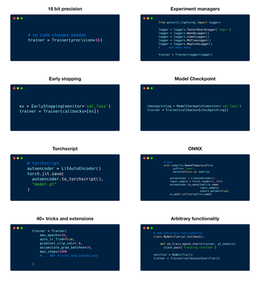
Because you are using this Lightning Trainer, you get some key advantages, such as model checkpointing and logging by default. You can also use 50+ best-practice tactics without needing to modify the model code, including multi-GPU training, model sharding, deep speed, quantization-aware training, early stopping, mixed precision, gradient clipping, and profiling.

Example commands for fine-tuning tactics, such as early stopping, model checkpoint, experiment managers, and more.
Figure 7. Fine-tuning tactics

Step 7: Inference and deployment

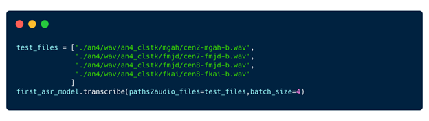
Now that you have a baseline model, inference it.

Figure 9. Run inference

Step 8: Pause session

Now that you have trained the model, you can pause the session and all the files that you need are persisted.

Screenshot shows the paused Grid session.
Figure 9. Monitor Grid session

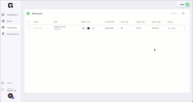
Paused sessions are free of charge and can be resumed as needed.

Conclusion

Now, you should have a better understanding of PyTorch Lightning, NGC, and Grid. You’ve fine-tuned your first NGC NeMo model and optimized it with Grid runs. We are excited to see what you do next with Grid and NGC.

Categories
Misc

Ray Tracing Gems II Available Today in Hardcover

Ray Tracing Games II is now available as a hardcover on Apress and Amazon.

Ray Tracing Games II is now available to download for free via Apress and Amazon and as a hardcover on Apress and Amazon as well. For those who love books as a physical medium, we recommend purchasing a copy for your home library, while also downloading the free PDF version for easy digital access on the go. 

This Open Access book is a must-have for anyone interested in real-time rendering. Ray tracing is the holy grail of gaming graphics, simulating the physical behavior of light to bring real-time, cinematic-quality rendering to even the most visually intense games. Ray tracing is also a fundamental algorithm used for architecture applications, visualization, sound simulation, deep learning, and more.

We’ve collaborated with our partners to make four limited edition versions of the book, featuring custom covers that highlight real-time ray tracing in Fortnite, Control, Watch Dogs: Legion, and Quake II RTX.

To win a limited edition print copy of Ray Tracing Gems II, enter the giveaway contest here: https://developer.nvidia.com/ray-tracing-gems-ii

Categories
Offsites

Detecting Abnormal Chest X-rays using Deep Learning

The adoption of machine learning (ML) for medical imaging applications presents an exciting opportunity to improve the availability, latency, accuracy, and consistency of chest X-ray (CXR) image interpretation. Indeed, a plethora of algorithms have already been developed to detect specific conditions, such as lung cancer, tuberculosis and pneumothorax. By virtue of being trained to detect a specific disease, however, the utility of these algorithms may be limited in a general clinical setting, where a wide variety of abnormalities could surface. For example, a pneumothorax detector is not expected to highlight nodules suggestive of cancer, and a tuberculosis detector may not identify findings specific to pneumonia. Since an initial triaging step is to determine whether a CXR contains any concerning abnormalities, a general-purpose algorithm that identifies X-rays containing any sort of abnormality could significantly facilitate the workflow. However, developing a classifier to detect any abnormality is challenging due to the ​​wide variety of abnormal findings that present on CXRs.

In “Deep Learning for Distinguishing Normal versus Abnormal Chest Radiographs and Generalization to Two Unseen Diseases Tuberculosis and COVID-19”, published in Scientific Reports, we present a model that can distinguish between normal and abnormal CXRs across multiple de-identified datasets and settings. We find that the model performs well on general abnormalities, as well as unseen examples of tuberculosis and COVID-19. We are also releasing our set of radiologists’ labels1 for the test set used in this study for the publicly available ChestX-ray14 dataset.

A Deep Learning System for Detecting Abnormal Chest X-rays
The deep learning system we used is based on the EfficientNet-B7 architecture, pre-trained on ImageNet. We trained the model using over 200,000 de-identified CXRs from the Apollo Hospitals in India. Each CXR was assigned a label of either “normal” or “abnormal” using a regular expression–based natural language processing approach on the associated radiology reports.

To evaluate how well the system generalizes to new patient populations, we compared its performance on two datasets consisting of a wide spectrum of abnormalities: the test split from the Apollo Hospitals dataset (DS-1), and the publicly available ChestX-ray14 (CXR-14). The labels for these two test sets were annotated for the purposes of this project by a group of US board-certified radiologists. The system achieved areas under the receiver operating characteristic curve (AUROC) of 0.87 on DS-1 and 0.94 on CXR-14 (higher is better).

Though the evaluations on DS-1 and CXR-14 contained a wide range of abnormalities, a possible use-case would be to utilize such an abnormality detector in novel or unforeseen settings with diseases that it had not encountered before. To evaluate the generalizability of the system to new patient populations and in the presence of diseases not seen in the training set, we used four de-identified datasets from three countries, including two publicly available tuberculosis datasets and two COVID-19 datasets from Northwestern Medicine. The system achieved AUCs of 0.95-0.97 in detecting tuberculosis, and 0.65-0.68 in detecting COVID-19. Because CXRs that are negative for these diseases could still contain other concerning abnormalities, we further evaluated the system for its ability to detect abnormalities more broadly (instead of disease positive vs. negative), finding AUCs of 0.91-0.93 for the tuberculosis dataset, and AUCs of 0.86 for the COVID-19 dataset.

The purpose of multiple evaluations (abnormality detection and disease detection) is the distinction between the two: a given disease can present with a certain abnormality or not; and a certain abnormality can arise from multiple diseases. Our study evaluates for both.

<!–

​​AUCs for Three Evaluation Setups
1. General Abnormalities 2. Unseen disease:

Tuberculosis

3. Unseen disease:

COVID-19

Detect abnormalities 0.87-0.94 0.91-0.93 0.86
Detect respective disease 0.95-0.97 0.65-0.68

–>

The large drop in performance for COVID-19 is because many cases flagged by the system as “positive” for abnormalities were negative for COVID-19, but nevertheless contained abnormal CXR findings that needed attention. This further highlights the usefulness of abnormality detectors even if disease-specific models are available.

In addition, it’s important to note that there is a difference between generalization to unseen diseases (i.e., tuberculosis and COVID-19) versus generalization to unseen CXR findings (e.g., pleural effusion, consolidation/infiltrate). In this study, we demonstrated the generalizability of the system to unseen diseases but not necessarily unseen CXR findings.

Sample chest X-rays of true and false positives, and true and false negatives for (A) general abnormalities, (B) tuberculosis, and (C) COVID-19. On each CXR, we outline in red the areas on which the model focused to identify abnormalities (i.e., the class activation map), and outline the regions of interest indicated by a radiologist in yellow.

Potential Benefits in the Clinic
To understand the potential utility of the deep learning model in improving clinical workflow, we simulated its use for case prioritization, where abnormal cases are “expedited” ahead of normal cases. In these simulations, the system reduced the turnaround time for abnormal cases by up to 28%. This reprioritization setup could be used to divert complex abnormal cases to cardiothoracic specialist radiologists, enable rapid triage of cases that may need urgent decisions, and provide the opportunity to batch negative CXRs for streamlined review.

Impact of a simulated deep learning model–based prioritization in comparison with random review order for (A) general abnormalities, (B) tuberculosis, and (C) COVID-19. The red bars indicate sequences of abnormal CXRs in red and normal CXRs in pink; a greater density of red towards the left indicates abnormal CXRs are reviewed sooner than normal ones. The histograms indicate the average improvement in turnaround time.

Additionally, we found that the system can be used as a pre-trained model to improve other ML algorithms for chest X-rays, especially when data is limited. For example, we used the normal/abnormal classifier in our recent study to detect pulmonary tuberculosis from chest X-rays. Abnormality and tuberculosis detectors can play a critical role in supporting early diagnosis in regions that lack access to resources like trained radiologists or molecular testing.

Sharing Improved Reference Standard Labels
Much work remains to be done to realize the potential of ML to aid chest X-ray interpretation around the world. In particular, obtaining high-quality labels on de-identified data can be a significant barrier to developing and evaluating ML algorithms in healthcare. To accelerate these efforts, we are expanding upon our previous label release by releasing the labels used in this study for the publicly available ChestX-ray14 dataset. We look forward to future machine learning projects by the community in this space.

AcknowledgementsKey contributors to this project at Google include Zaid Nabulsi, Andrew Sellergren‎, Shahar Jamshy, Charles Lau, Eddie Santos, Atilla P. Kiraly, Wenxing Ye, Jie Yang, Rory Pilgrim, Sahar Kazemzadeh, Jin Yu, Greg S. Corrado, Lily Peng, Krish Eswaran, Daniel Tse, Neeral Beladia, Yun Liu, Po-Hsuan Cameron Chen, Shravya Shetty. Significant contributions and input were also made by radiologist collaborators Sreenivasa Raju Kalidindi, Mozziyar Etemadi, Florencia Garcia Vicente, David Melnick. For the CXR-14 dataset, we thank the NIH Clinical Center for making it publicly available. For tuberculosis data collection, thanks go to Sameer Antani, Stefan Jaeger, Sema Candemir, Zhiyun Xue, Alex Karargyris, George R. Thomas, Pu-Xuan Lu, Yi-Xiang Wang, Michael Bonifant, Ellan Kim, Sonia Qasba, and Jonathan Musco. The authors would also like to acknowledge many members of the Google Health Radiology and labeling software teams, in particular Shruthi Prabhakara, Scott McKinney, and Akib Uddin. Sincere appreciation also goes to the radiologists who enabled this work with their image interpretation and annotation efforts throughout the study; Jonny Wong for coordinating the imaging annotation work; Gavin Bee, Mikhail Fomitchev, Shabir Adeel, Jeff Bertram, and Benedict Noero for data releasing; David F. Steiner, Kunal Nagpal, and Michael D. Howell for providing feedback on the manuscript; Craig Mermel, Lauren Winer, Johnny Luu, Adrienne Welch, Annisah Um’rani, and Ashley Zlatinov for feedback on the blogpost.


1Labels include atelectasis, cardiomegaly, effusion, infiltration, mass, nodule, pneumonia, pneumothorax, consolidation, edema, emphysema, fibrosis, pleural thickening, hernia, other abnormality, and normal vs abnormal. 

Categories
Misc

What Is Accelerated Computing?

Accelerated computing is humming in the background, making life better even on a quiet night at home. It prevents credit card fraud when you buy a movie to stream. It recommends a dinner you might like and arranges a fast delivery. Maybe it even helped the movie’s director win an Oscar for stunning visuals. So, Read article >

The post What Is Accelerated Computing? appeared first on The Official NVIDIA Blog.

Categories
Misc

Machine Learning Frameworks Interoperability, Part 3: Zero-Copy in Action using an E2E Pipeline

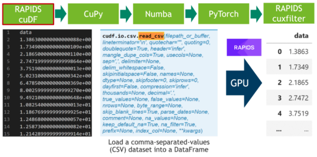
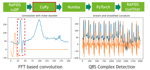
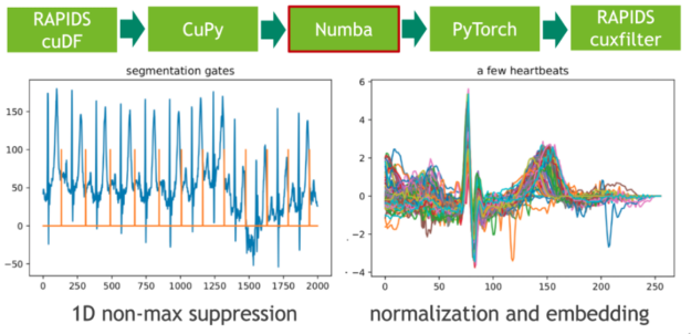
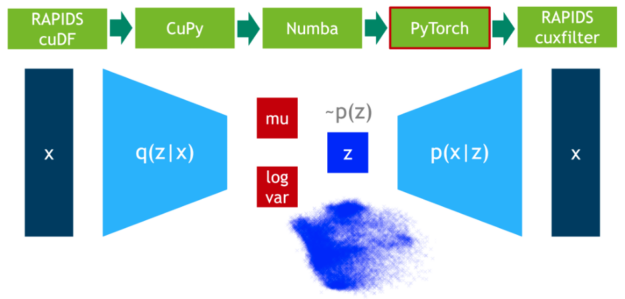
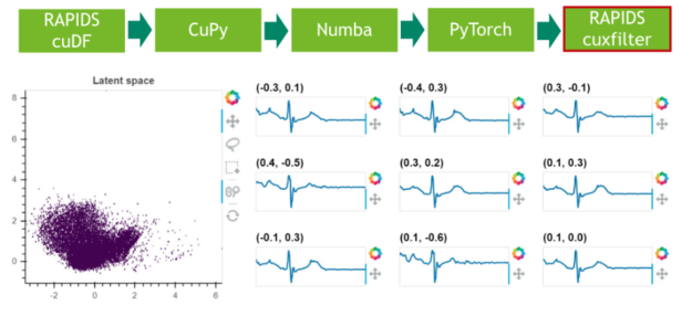
Machine Learning Frameworks Interoperability part 3 covers on the implementation of an end-to-end pipeline demonstrating the discussed techniques for optimal data transfer across data science frameworks.

Introduction

Efficient pipeline design is crucial for data scientists. When composing complex end-to-end workflows, you may choose from a wide variety of building blocks, each of them specialized for a dedicated task. Unfortunately, repeatedly converting between data formats is an error-prone and performance-degrading endeavor. Let’s change that!

In this blog series, we discuss different aspects of efficient framework interoperability:

  • In the first post, we discussed pros and cons of distinct memory layouts as well as memory pools for asynchronous memory allocation to enable zero-copy functionality.
  • In the second post, we highlighted bottlenecks occurring during data loading/transfers and how to mitigate them using Remote Direct Memory Access (RDMA) technology.
  • In this post, we dive into the implementation of an end-to-end pipeline demonstrating the discussed techniques for optimal data transfer across data science frameworks.

To learn more on framework interoperability, check out our presentation at NVIDIA’s GTC 2021 Conference.

Let’s dive into the implementation details of a fully functional pipeline for:

  • Parsing of 20 hours of continuously measured electrocardiograms (ECGs) from plain CSV files.
  • Unsupervised segmentation of bespoke ECG stream into individual heart beats using traditional signal processing techniques.
  • Subsequent training of a variational autoencoder (VAE) for outlier detection.
  • Final visualization of the results.

For each of the previous steps, a different data science library is used, so making efficient data conversion a crucial task. Most importantly, you should avoid costly CPU roundtrips when copying data from one GPU-based framework to another.

Zero-Copy in Action: End-to-End pipeline

Enough talk! Let’s see framework interoperability in action. In the following, we will discuss the end-to-end pipeline step by step. If you are an impatient person, you can directly download the full Jupyter notebook here. The source code can be executed from within a recent RAPIDS docker container. 

Step 1: Data loading

In the first step, we download 20 hours of electrocardiograms as a CSV file and write it to disk (see Cell 1). After, we parse the 500 MB of scalar values from the CSV file and transfer them directly to the GPU using RAPIDS’ blazing fast CSV reader (see Cell 2). Now, the data resides on the GPU and will stay there until the very end. Next, we plot the whole time series consisting of 20 million scalar data points using the cuxfilter (ku-cross-filter) framework (see Cell 3).

A table of floating-point numbers in CSV format, the API call for cudf.io.csv.read_csv, as well as the resulting data frame in RAPIDS.
Figure 1:  Parsing comma-separated values (CSV) using the RAPIDS CSV parser.

Step 2: Data segmentation

In the next step, we segment the 20 hours ECG into individual heartbeats using traditional signal processing techniques. We achieve that by convolving the ECG stream with the second derivative of a Gaussian distribution, also known as Ricker wavelet, in order to isolate the corresponding frequency band of the initial peak in a prototypical heartbeat. Both the sampling of the wavelet as well as the FFT-based convolution are facilitated using CuPy, a CUDA-accelerated library for dense linear algebra and array operations. As a direct result, the RAPIDS cuDF dataframe storing the ECG data has to be converted to a CuPy array using DLPack as a zero-copy mechanism. 

The left panel depicts a single heartbeat and a Ricker wavelet. The right panel depicts 13 continuously measured heartbeats and the corresponding output of the convolution with the Ricker wavelet.
Figure 2: Convolving the electrocardiogram (ECG) stream with a Ricker wavelet of fixed-width using CuPy.

The feature response (result) of the convolution measures the presence of a fixed frequency content for each position in the stream. Note that we have chosen the wavelet in a way so that local maxima correspond to the initial peak of a heartbeat. 

Step 3: Local maxima detection

In the next step, we map these extremal points to a binary gate using a 1D variant of non-maximum suppression (NMS). NMS determines for every position in the stream if the corresponding value is the maximum in a predefined window (neighborhood). A CUDA implementation of this embarrassingly parallel problem is straightforward. In our example, we use the just-in-time compiler Numba to allow for seamless Python integration. Both Numba and Cupy implement the CUDA array interface as a zero-copy mechanism and thus the explicit cast from CuPy arrays to Numba device arrays can be fully avoided. 

The left panel depicts the segmentation gates for 13 continuously measured heartbeats coming from the 1D non-maximum suppression. The right panel visualizes a few approximately aligned heartbeats embedded in a vector of length 256.
Figure 3:  1D non-maximum suppression and embedding of heartbeats using Numba JIT.

The length of each heartbeat is determined by computing the adjacent difference (finite step derivative) of the gate positions. We facilitate this by filtering the index domain with the predicate gate==1 followed by a call to cupy.diff(). The resulting histogram depicts the length distribution.

Step 4: Candidate pruning and embedding

We intend to train a (convolutional) Variational Autoencoder (VAE) on the set of heartbeats using a fixed-length input matrix. The embedding of heartbeats in a vector of zeros can be realized with a CUDA kernel. Here, we again use Numba for both candidate pruning and embedding. 

Step 5: Outliers detection

In this step, we train the VAE model on 75% of the data. DLPack is used again as the zero-copy mechanism to map the CuPy data matrix to a PyTorch tensor.

The network topology of a variational autoencoder with an approximately isotropic point cloud below the (middle) latent layer.
Figure 4: Training a variational autoencoder using PyTorch.

Step 6: Results visualization

In a final step, we visualize the latent space of the remaining 25% of the data.

An approximately isotropic Gaussian point cloud in the 2D plane and 9 (fake) heart beats generated with the decoder of the autoencoder.
Figure 5: Sampling and visualizing the latent space using RAPIDS cuxfilter.

Conclusion

A key takeaway from this and the preceding blog posts is that interoperability is crucial for the design of efficient data pipelines. Copy-and-converting data between different frameworks is an expensive and incredibly time-consuming task that adds zero value to data science pipelines. Data science workloads are becoming increasingly complex, and the interaction between multiple software libraries is common practice. DLPack and the CUDA Array Interface are the de facto data format standards that guarantee zero-copy data exchange among GPU-based frameworks.

Support for external memory managers is a nice-to-have feature to consider when appraising which software libraries your pipeline will use. For instance, if your task requires both DataFrame and array data manipulation, a great choice of libraries is RAPIDS cuDF + CuPy. They both benefit from GPU acceleration, support DLPack to exchange data with zero-copy, and share the same memory manager, RMM. Alternatively, RAPIDS cuDF + JAX would also be an excellent option. Nevertheless, the latter combination might require extra development efforts to leverage memory usage because of JAX’s lack of support for external memory allocators.

Data loading and data transfer bottlenecks are frequent when dealing with large datasets. NVIDIA GPUDirect technology comes to the rescue, supporting moving data into or out of the GPU memory without burdening the CPU and reducing to one the number of data copies needed when transferring data between GPUs on different nodes.