
 Technical overview of the Nsight DL Designer tool to help ease the process of performant model design.
NVIDIA Nsight Deep Learning Designer is a new tool that helps ease the process of performant model design. DL Designer provides valuable insights into the structure of the model, and how well it performs on NVIDIA hardware. Models can be created with a user-friendly, drag-and-drop interface that features nodes for all of the commonly used operators available in the most popular deep learning frameworks.
Performance profiling
Understanding the performance characteristics of a model is essential right from the outset. After the model is designed, you can profile it for performance.
To select and view the latest profiling report, choose Launch Inference, View, Inference Run Logger.
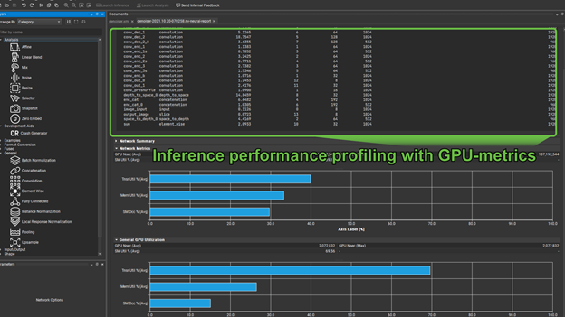
This is divided into two major sections. The first, shown previously, gives you a table of operators, their hyperparameters, and execution times. These are, by default, listed in order of priority to optimize (akin to how nvprof lists kernels in order of optimization priority).
An important question for any model running on NVIDIA hardware, for both training and inference is, “Is this model using Tensor Cores”? The second part of the profiling report shows the utilization of Tensor Cores.
There are two groups of graphs here, the first gives you the Tensor Core utilization, along with memory throughput, and SM occupancy for the entire network. The second gives these same metrics for an individually selected operator from the preceding list. In cases where Tensor Core utilization is not meaningful, for example in the case of a pooling operator, the Tensor Core utilization shows as zero.
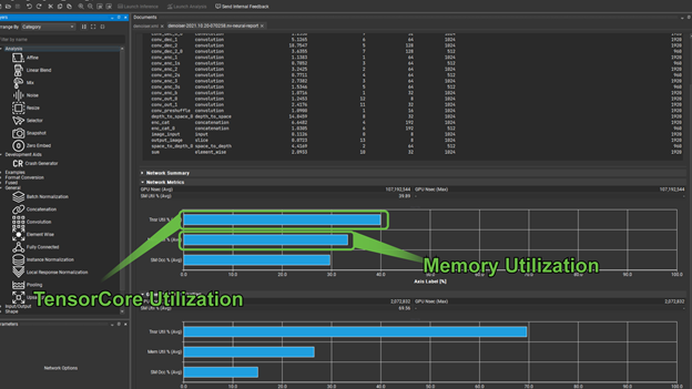
Memory utilization can quickly tell you if you are memory-bound. In cases such as this, it is prudent to look for opportunities to fuse operators where appropriate to use faster memory. Training time can be hugely reduced if you use the GPU hardware effectively. When training large models, or using cloud-based services, this can quickly translate into greatly reduced production costs.
Training the model
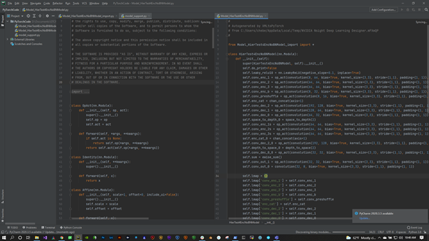
After you have profiled your model for performance improvements, you can export the model to PyTorch and perform training. Improvement areas can include ensuring FP16, when NHWC layout is used and you have at least multiples of eight input/output channels for your conv2d convolutions.
To export to PyTorch, choose File, Export, Generate PyTorch Files (Figure 3).
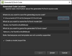
Exporting your model to PyTorch gives you a few options to check the names of the model, and files that are selected for you. But, you must specify an output directory for your PyTorch files, which consists of a trainable model and some utility methods to work with it.
To export to PyTorch, you must have a Python 3 environment in your PATH environment variable and the following modules:
- PyTorch
- Numpy
- Pillow
- Matplotlib
- Fastprogress
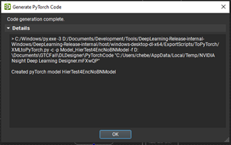
Upon successful generation, close the Code generation complete dialog box.
Analyzing the model
Now your code is ready to work with! The next step is to get it trained and the weights loaded back into DL Designer so that you can analyze how well the model is performing the task for which it was designed.
The model here is a denoiser model. It is in the samples that you can try for yourself. The first thing to do is load it into DL Designer. Next get and apply the weights that you got from the training in PyTorch.
To configure the trained model, choose Tools, Network Settings.
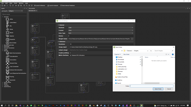
The first thing to look at is the Weights Folder. Select the directory where you output your trained weights. DL Designer picks these up and applies them to the appropriate operators.
Also, make sure that you are set to FP16, NHWC layout, and the CUDA backend. To use the fast Tensor Cores for operations such as convolutions and GEMMs (matrix multiplications), use FP16. To get the fastest throughput, use NHWC.
Now, you can begin performing some visual analysis on the model. Before you do that, use some of the DL Designer analysis features and add a few handy nodes to the trained model to help you evaluate its performance as a denoiser.
Analysis layers
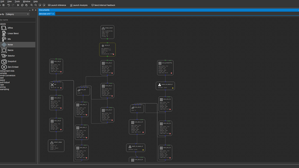
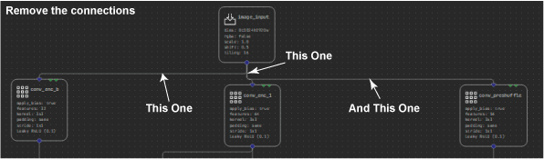
Start by expanding the Analysis section of the Layers palette. The first new layer to add is the Noise layer. This helps you inject some noise into the input image, so that you can evaluate how well the denoiser is reconstructing the image without it. To do this, first select and delete the connections between Input_image and the three nodes it connects with: conv_enc_b, conv_enc_1, and conv_preshuffle.
Now select and shift the image input node up a touch so that you can fit the noise layer in between. Finally, connect the input _image node to the new Noise layer, then connect the new layer to the three nodes that were previously connected from the image input. When you run this model, you can control how much noise to add to the image.
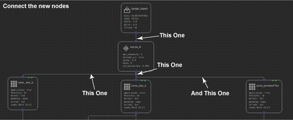
Before you run the analysis, there is one more node that you might find useful: the Mix node. This node enables you to compare the final denoised output with the original input, before the noise was added. As you see, you can perform this comparison in a variety of ways that give you a good idea as to how well your model is performing.
Delete the connection between conv_out_0 and output_image and then insert the Mix node in between these two, much like you did with the noise node by replacing the connections. I recommend caution as the mix node actually has two inputs.
You have already specified conv_out_0 as one input. Now add the other input to connect to the output of the original image layer, right at the top of the model, before you add the noise.
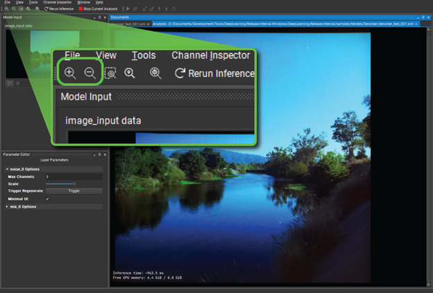
So far, you’ve added handy utilities to help analyze the model. At this point, save your model as denoiser_analyze.xml (or something similar) and choose Launch Analysis to see the model in action. Here is a quick breakdown of the user interface:
- image_input_data—Right-click and choose Open Image Input to browse for a JPG or PNG file for use as the original input. When you choose Ok, the model springs into life and the output of the model is displayed in the central panel.
- Noise and Mix—Options for the two analysis layers just added.
- Network overview—The graph of nodes as they are being executed by the model inference.
Customizing design inspection
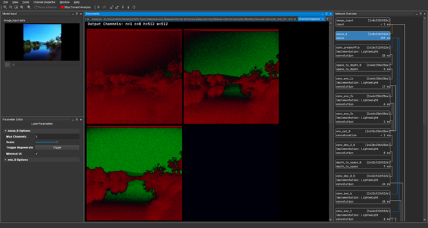
To continue, double-click on the Noise layer, which is the second layer down under Network Overview. Through the Channel Inspector under this tab, you can see the individual channels of the tensors that are produced during inference, which are the hidden layers. With the Noise layer channels in view, you can now go back to the noise layer options at the bottom right of the screen. Drag the Scale slider a little to the right and see the amount of noise showing on the image input increase.
Under Channel Inspector, double-click the conv_enc_2s layer and load the channels of that hidden layer. This is showing the results of the convolution operation at the point during inference.
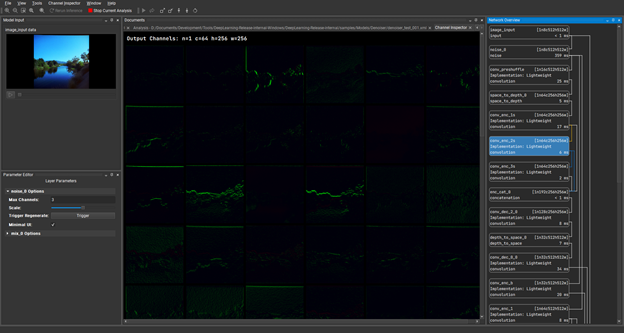
The features in these channels are a little faint, but you can boost them a bit by choosing the scale up icon (Figure 12).
This gives you a better idea of how these layers are performing and you can see clearly that there is nothing collapsing here. You have got strong signals propagating through the model. Any data displayed as green is positive in value and any data displayed as red is negative.
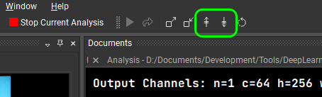
You can also shift the displayed values with the shift buttons, enabling you to push everything to display as positive or negative values.
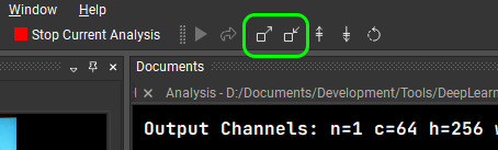
Have a look at the final output of the model and compare it with the original input. This is where the mix layer comes into play. Close down the channel inspector and look at the image output again. Use the Zoom button in the top left corner to make that output fill the user interface so that you can really see what is going on.
Under Mix Layer in the bottom left, change Mix Choice to V Split. When you drag the Mix Amount slider from left to right, you can see that you are actually getting a split screen between the original input and the reconstructed, denoised output. It is certainly useful, but the effect is quite subtle.
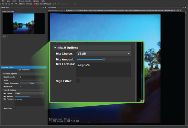
You could conclude that the denoiser is serving its purpose, but the differences are subtle. What can you do to get a clearer idea about which image parts are performing better than others?
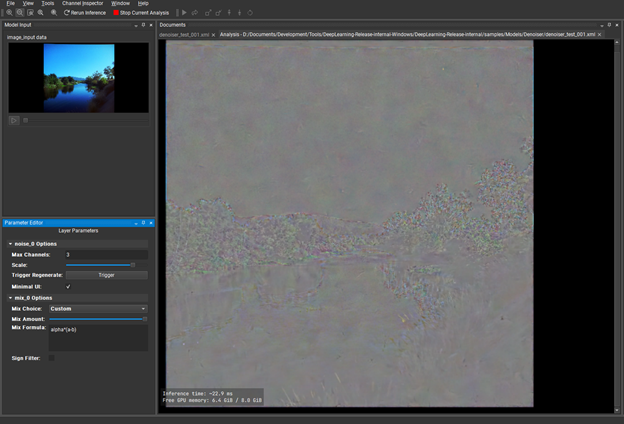
Under Mix Layer, change Mix Choice to Custom. For Mix Formula, replace the existing expression with: alpha * (a-b). The alpha keyword is effectively the normalized value of the slider and a and b are the two inputs of the layer. This creates a visual diff of the input and output that you can visually boost with the mix slider and tells you where there are fundamental differences between input and output.
This is the sort of thing that tells you, “Yes, your model is fine.” Or maybe, “You should revisit your architecture or training data.”
Conclusion
NVNsight DL Designer provides even more features, such as NvNeural, a highly optimized inference engine with an extensible plugin-based architecture that enables you to implement your own layer types.
Together with the design and analysis tools, DL Designer is a highly interactive and versatile solution to model design, reducing coding errors, and complexities to focus more on the capabilities and performance of your models.
For more information, see the following resources:
- Download the latest release of Nsight DL Designer.
- Read the Nsight DL Designer documentation.
- Ask questions or give feedback on the Nsight Systems forums.
- Get the Nsight Developer Tools free as a registered NVIDIA Developer Program member.
- You can also get the tools as part of the NVIDIA CUDA toolkit.