
Month: November 2021
Despite the success and widespread adoption of smartphones, using them to compose longer pieces of text is still quite cumbersome. As one writes, grammatical errors can often creep into the text (especially undesirable in formal situations), and correcting these errors can be time consuming on a small display with limited controls.
To address some of these challenges, we are launching a grammar correction feature that is directly built into Gboard on Pixel 6 that works entirely on-device to preserve privacy, detecting and suggesting corrections for grammatical errors while the user is typing. Building such functionality required addressing a few key obstacles: memory size limitations, latency requirements, and handling partial sentences. Currently, the feature is capable of correcting English sentences (we plan to expand to more languages in the near future) and available on almost any app with Gboard1.
 |
| Gboard suggests how to correct an ungrammatical sentence as the user types. |
Model Architecture
We trained a sequence-to-sequence neural network to take an input sentence (or a sentence prefix) and output the grammatically correct version — if the original text is already grammatically correct, the output of the model is identical to its input, indicating that no corrections are needed. The model uses a hybrid architecture that combines a Transformer encoder with an LSTM decoder, a combination that provides a good balance of quality and latency.
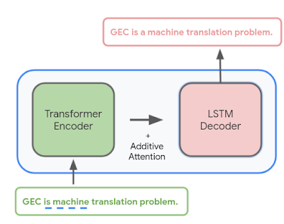 |
| Overview of the grammatical error correction (GEC) model architecture. |
Mobile devices are constrained by limited memory and computational power, which make it more difficult to build a high quality grammar checking system. There are a few techniques we use to build a small, efficient, and capable model.
- Shared embedding: Because the input and output of the model are structurally similar (e.g., both are text in the same language), we share some of the model weights between the Transformer encoder and the LSTM decoder, which reduces the model file size considerably without unduly affecting accuracy.
- Factorized embedding: The model splits a sentence into a sequence of predefined tokens. To achieve good quality, we find that it is important to use a large vocabulary of predefined tokens, however, this substantially increases the model size. A factorized embedding separates the size of the hidden layers from the size of the vocabulary embedding. This enables us to have a model with a large vocabulary without significantly increasing the number of total weights.
- Quantization: To reduce the model size further, we perform post-training quantization, which allows us to store each 32-bit floating point weight using only 8-bits. While this means that each weight is stored with lower fidelity, nevertheless, we find that the quality of the model is not materially affected.
By employing these techniques, the resulting model takes up only 20MB of storage and performs inference on 60 input characters under 22ms on the Google Pixel 6 CPU.
Training the Model
In order to train the model, we needed training data in the form of <original, corrected> text pairs.
One possible approach to generating a small on-device model would be to use the same training data as a large cloud-based grammar model. While this data produces a reasonably high quality on-device model, we found that using a technique called hard distillation to generate training data that is better-matched to the on-device domain yields even better quality results.
Hard distillation works as follows: We first collected hundreds of millions of English sentences from across the public web. We then used the large cloud-based grammar model to generate grammar corrections for those sentences. This training dataset of <original, corrected> sentence pairs is then used to train a smaller on-device model that can correct full sentences. We found that the on-device model built from this training dataset produces significantly higher quality suggestions than a similar-sized on-device model built on the original data used to train the cloud-based model.
Before training the model from this data, however, there is another issue to address. To enable the model to correct grammar as the user types (an important capability of mobile devices) it needs to be able to handle sentence prefixes. While this enables grammar correction when the user has only typed part of a sentence, this capability is particularly useful in messaging apps, where the user often omits the final period in a sentence and presses the send button as soon as they finish typing. If grammar correction is only triggered on complete sentences, it might miss many errors.
This raises the question of how to decide whether a given sentence prefix is grammatically correct. We used a heuristic to solve this — if a given sentence prefix can be completed to form a grammatically correct sentence, we then consider it grammatically correct. If not, it is assumed to be incorrect.
| What the user has typed so far | Suggested grammar correction | |
| She puts a lot | ||
| She puts a lot of | ||
| She puts a lot of effort | ||
| She puts a lot of effort yesterday | Replace “puts” with “put in”. |
| GEC on incomplete sentences. There is no correction for valid sentence prefixes. |
We created a second dataset suitable for training a large cloud-based model, but this time focusing on sentence prefixes. We generated the data using the aforementioned heuristic by taking the <original, corrected> sentence pairs from the cloud-based model’s training dataset and randomly sampling aligned prefixes from them.
For example, given the <original, corrected> sentence pair:
Original sentence: She puts a lot of effort yesterday afternoon.
Corrected sentence: She put in a lot of effort yesterday afternoon.
We might sample the following prefix pairs:
Original prefix: She puts
Corrected prefix: She put in
Original prefix: She puts a lot of effort yesterday
Corrected prefix: She put in a lot of effort yesterday
We then autocompleted each original prefix to a full sentence using a neural language model (similar in spirit to that used by SmartCompose). If a full-sentence grammar model finds no errors in the full sentence, then that means there is at least one possible way to complete this original prefix without making any grammatical errors, so we consider the original prefix to be correct and output <original prefix, original prefix> as a training example. Otherwise, we output <original prefix, corrected prefix>. We used this training data to train a large cloud-based model that can correct sentence prefixes, then used that model for hard distillation, generating new <original, corrected> sentence prefix pairs that are better-matched to the on-device domain.
Finally, we constructed the final training data for the on-device model by combining these new sentence prefix pairs with the full sentence pairs. The on-device model trained on this combined data is then capable of correcting both full sentences as well as sentence prefixes.
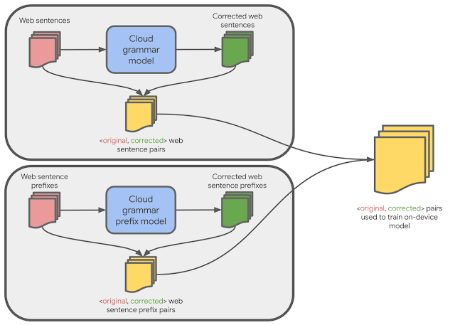 |
| Training data for the on-device model is generated from cloud-based models. |
Grammar Correction On-Device
Gboard sends a request to the on-device grammar model whenever the user has typed more than three words, whether the sentence is completed or not. To provide a quality user experience, we underline the grammar mistakes and provide replacement suggestions when the user interacts with them. However, the model outputs only corrected sentences, so those need to be transformed into replacement suggestions. To do this, we align the original sentence and the corrected sentence by minimizing the Levenshtein distance (i.e., the number of edits that are needed to transform the original sentence to the corrected sentence).
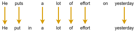 |
| Extracting edits by aligning the corrected sentence to the original sentence. |
Finally, we transform the insertion edits and deletion edits to be replacement edits. In the above example, we transform the suggested insertion of “in” to be an edit that suggests replacing “puts” with “put in”. And we similarly suggest replacing “effort on” with “effort”.
Conclusion
We have built a small high-quality grammar correction model by designing a compact model architecture and leveraging a cloud-based grammar system during training via hard distillation. This compact model enables users to correct their text entirely on their own device without ever needing to send their keystrokes to a remote server.
Acknowledgements
We gratefully acknowledge the key contributions of the other team members, including Abhanshu Sharma, Akshay Kannan, Bharath Mankalale, Chenxi Ni, Felix Stahlberg, Florian Hartmann, Jacek Jurewicz, Jayakumar Hoskere, Jenny Chin, Kohsuke Yatoh, Lukas Zilka, Martin Sundermeyer, Matt Sharifi, Max Gubin, Nick Pezzotti, Nithi Gupta, Olivia Graham, Qi Wang, Sam Jaffee, Sebastian Millius, Shankar Kumar, Sina Hassani, Vishal Kumawat, and Yuanbo Zhang, Yunpeng Li, Yuxin Dai. We would also like to thank Xu Liu and David Petrou for their support.
1The feature will eventually be available in all apps with Gboard, but is currently unavailable for those in WebView. ↩

Emotions are a key aspect of social interactions, influencing the way people behave and shaping relationships. This is especially true with language — with only a few words, we’re able to express a wide variety of subtle and complex emotions. As such, it’s been a long-term goal among the research community to enable machines to understand context and emotion, which would, in turn, enable a variety of applications, including empathetic chatbots, models to detect harmful online behavior, and improved customer support interactions.
In the past decade, the NLP research community has made available several datasets for language-based emotion classification. The majority of those are constructed manually and cover targeted domains (news headlines, movie subtitles, and even fairy tales) but tend to be relatively small, or focus only on the six basic emotions (anger, surprise, disgust, joy, fear, and sadness) that were proposed in 1992. While these emotion datasets enabled initial explorations into emotion classification, they also highlighted the need for a large-scale dataset over a more extensive set of emotions that could facilitate a broader scope of future potential applications.
In “GoEmotions: A Dataset of Fine-Grained Emotions”, we describe GoEmotions, a human-annotated dataset of 58k Reddit comments extracted from popular English-language subreddits and labeled with 27 emotion categories . As the largest fully annotated English language fine-grained emotion dataset to date, we designed the GoEmotions taxonomy with both psychology and data applicability in mind. In contrast to the basic six emotions, which include only one positive emotion (joy), our taxonomy includes 12 positive, 11 negative, 4 ambiguous emotion categories and 1 “neutral”, making it widely suitable for conversation understanding tasks that require a subtle differentiation between emotion expressions.
We are releasing the GoEmotions dataset along with a detailed tutorial that demonstrates the process of training a neural model architecture (available on TensorFlow Model Garden) using GoEmotions and applying it for the task of suggesting emojis based on conversational text. In the GoEmotions Model Card we explore additional uses for models built with GoEmotions, as well as considerations and limitations for using the data.
 |
| This text expresses several emotions at once, including excitement, approval and gratitude. |
 |
| This text expresses relief, a complex emotion conveying both positive and negative sentiment. |
 |
| This text conveys remorse, a complex emotion that is expressed frequently but is not captured by simple models of emotion. |
Building the Dataset
Our goal was to build a large dataset, focused on conversational data, where emotion is a critical component of the communication. Because the Reddit platform offers a large, publicly available volume of content that includes direct user-to-user conversation, it is a valuable resource for emotion analysis. So, we built GoEmotions using Reddit comments from 2005 (the start of Reddit) to January 2019, sourced from subreddits with at least 10k comments, excluding deleted and non-English comments.
To enable building broadly representative emotion models, we applied data curation measures to ensure the dataset does not reinforce general, nor emotion-specific, language biases. This was particularly important because Reddit has a known demographic bias leaning towards young male users, which is not reflective of a globally diverse population. The platform also introduces a skew towards toxic, offensive language. To address these concerns, we identified harmful comments using predefined terms for offensive/adult and vulgar content, and for identity and religion, which we used for data filtering and masking. We additionally filtered the data to reduce profanity, limit text length, and balance for represented emotions and sentiments. To avoid over-representation of popular subreddits and to ensure the comments also reflect less active subreddits, we also balanced the data among subreddit communities.
We created a taxonomy seeking to jointly maximize three objectives: (1) provide the greatest coverage of the emotions expressed in Reddit data; (2) provide the greatest coverage of types of emotional expressions; and (3) limit the overall number of emotions and their overlap. Such a taxonomy allows data-driven fine-grained emotion understanding, while also addressing potential data sparsity for some emotions.
Establishing the taxonomy was an iterative process to define and refine the emotion label categories. During the data labeling stages, we considered a total of 56 emotion categories. From this sample, we identified and removed emotions that were scarcely selected by raters, had low interrater agreement due to similarity to other emotions, or were difficult to detect from text. We also added emotions that were frequently suggested by raters and were well represented in the data. Finally, we refined emotion category names to maximize interpretability, leading to high interrater agreement, with 94% of examples having at least two raters agreeing on at least 1 emotion label.
The published GoEmotions dataset includes the taxonomy presented below, and was fully collected through a final round of data labeling where both the taxonomy and rating standards were pre-defined and fixed.
 |
| GoEmotions taxonomy: Includes 28 emotion categories, including “neutral”. |
<!–
| Positive | Negative | Ambiguous | ||
| admiration 👏 | joy 😃 | anger 😡 | grief 😢 | confusion 😕 |
| amusement 😂 | love ❤️ | annoyance 😒 | nervousness 😬 | curiosity 🤔 |
| approval 👍 | optimism 🤞 | disappointment | remorse 😔 | realization 💡 |
| caring 🤗 | pride 😌 | disapproval 👎 | sadness 😞 | surprise 😲 |
| desire 😍 | relief 😅 | disgust 🤮 | ||
| excitement 🤩 | embarrassment 😳 | |||
| gratitude 🙏 | fear 😨 | |||
–>
Data Analysis and Results
Emotions are not distributed uniformly in the GoEmotions dataset. Importantly, the high frequency of positive emotions reinforces our motivation for a more diverse emotion taxonomy than that offered by the canonical six basic emotions.

To validate that our taxonomic choices match the underlying data, we conduct principal preserved component analysis (PPCA), a method used to compare two datasets by extracting linear combinations of emotion judgments that exhibit the highest joint variability across two sets of raters. It therefore helps us uncover dimensions of emotion that have high agreement across raters. PPCA was used before to understand principal dimensions of emotion recognition in video and speech, and we use it here to understand the principal dimensions of emotion in text.
We find that each component is significant (with p-values < 1.5e-6 for all dimensions), indicating that each emotion captures a unique part of the data. This is not trivial, since in previous work on emotion recognition in speech, only 12 out of 30 dimensions of emotion were found to be significant.
We examine the clustering of the defined emotions based on correlations among rater judgments. With this approach, two emotions will cluster together when they are frequently co-selected by raters. We find that emotions that are related in terms of their sentiment (negative, positive and ambiguous) cluster together, despite no predefined notion of sentiment in our taxonomy, indicating the quality and consistency of the ratings. For example, if one rater chose “excitement” as a label for a given comment, it is more likely that another rater would choose a correlated sentiment, such as “joy”, rather than, say, “fear”. Perhaps surprisingly, all ambiguous emotions clustered together, and they clustered more closely with positive emotions.

Similarly, emotions that are related in terms of their intensity, such as joy and excitement, nervousness and fear, sadness and grief, annoyance and anger, are also closely correlated.

Our paper provides additional analyses and modeling experiments using GoEmotions.
Future Work: Alternatives to Human-Labeling
While GoEmotions offers a large set of human-annotated emotion data, additional emotion datasets exist that use heuristics for automatic weak-labeling. The dominant heuristic uses emotion-related Twitter tags as emotion categories, which allows one to inexpensively generate large datasets. But this approach is limited for multiple reasons: the language used on Twitter is demonstrably different than many other language domains, thus limiting the applicability of the data; tags are human generated, and, when used directly, are prone to duplication, overlap, and other taxonomic inconsistencies; and the specificity of this approach to Twitter limits its applications to other language corpora.
We propose an alternative, and more easily available heuristic in which emojis embedded in user conversation serve as a proxy for emotion categories. This approach can be applied to any language corpora containing a reasonable occurence of emojis, including many that are conversational. Because emojis are more standardized and less sparse than Twitter-tags, they present fewer inconsistencies.
Note that both of the proposed approaches — using Twitter tags and using emojis — are not directly aimed at emotion understanding, but rather at variants of conversational expression. For example, in the conversation below, 🙏 conveys gratitude, 🎂 conveys a celebratory expression, and 🎁 is a literal replacement for ‘present’. Similarly, while many emojis are associated with emotion-related expressions, emotions are subtle and multi-faceted, and in many cases no one emoji can truly capture the full complexity of an emotion. Moreover, emojis capture varying expressions beyond emotions. For these reasons, we consider them as expressions rather than emotions.

This type of data can be valuable for building expressive conversational agents, as well as for suggesting contextual emojis, and is a particularly interesting area of future work.
Conclusion
The GoEmotions dataset provides a large, manually annotated, dataset for fine-grained emotion prediction. Our analysis demonstrates the reliability of the annotations and high coverage of the emotions expressed in Reddit comments. We hope that GoEmotions will be a valuable resource to language-based emotion researchers, and will allow practitioners to build creative emotion-driven applications, addressing a wide range of user emotions.
Acknowledgements
This blog presents research done by Dora Demszky (while interning at Google), Dana Alon (previously Movshovitz-Attias), Jeongwoo Ko, Alan Cowen, Gaurav Nemade, and Sujith Ravi. We thank Peter Young for his infrastructure and open sourcing contributions. We thank Erik Vee, Ravi Kumar, Andrew Tomkins, Patrick Mcgregor, and the Learn2Compress team for support and sponsorship of this research project.
An approach commonly used to train agents for a range of applications from robotics to chip design is reinforcement learning (RL). While RL excels at discovering how to solve tasks from scratch, it can struggle in training an agent to understand the reversibility of its actions, which can be crucial to ensure that agents behave in a safe manner within their environment. For instance, robots are generally costly and require maintenance, so one wants to avoid taking actions that might lead to broken components. Estimating if an action is reversible or not (or better, how easily it can be reversed) requires a working knowledge of the physics of the environment in which the agent is operating. However, in the standard RL setting, agents do not possess a model of the environment sufficient to do this.
In “There Is No Turning Back: A Self-Supervised Approach to Reversibility-Aware Reinforcement Learning”, accepted at NeurIPS 2021, we present a novel and practical way of approximating the reversibility of agent actions in the context of RL. This approach, which we call Reversibility-Aware RL, adds a separate reversibility estimation component to the RL procedure that is self-supervised (i.e., it learns from unlabeled data collected by the agents). It can be trained either online (jointly with the RL agent) or offline (from a dataset of interactions). Its role is to guide the RL policy towards reversible behavior. This approach increases the performance of RL agents on several tasks, including the challenging Sokoban puzzle game.
Reversibility-Aware RL
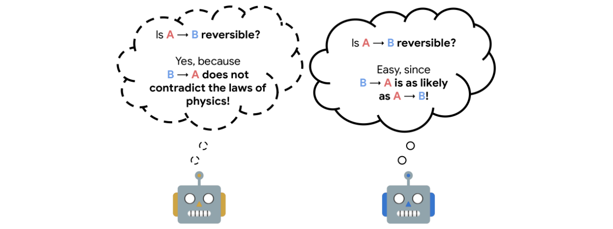
The reversibility component added to the RL procedure is learned from interactions, and crucially, is a model that can be trained separate from the agent itself. The model training is self-supervised and does not require that the data be labeled with the reversibility of the actions. Instead, the model learns about which types of actions tend to be reversible from the context provided by the training data alone.We call the theoretical explanation for this empirical reversibility, a measure of the probability that an event A precedes another event B, knowing that A and B both happen. Precedence is a useful proxy for true reversibility because it can be learned from a dataset of interactions, even without rewards.
Imagine, for example, an experiment where a glass is dropped from table height and when it hits the floor it shatters. In this case, the glass goes from position A (table height) to position B (floor) and regardless of the number of trials, A always precedes B, so when randomly sampling pairs of events, the probability of finding a pair in which A precedes B is 1. This would indicate an irreversible sequence. Assume, instead, a rubber ball was dropped instead of the glass. In this case, the ball would start at A, drop to B, and then (approximately) return to A. So, when sampling pairs of events, the probability of finding a pair in which A precedes B would only be 0.5 (the same as the probability that a random pair showed B preceding A), and would indicate a reversible sequence.
 |
| Reversibility estimation relies on the knowledge of the dynamics of the world. A proxy to reversibility is precedence, which establishes which of two events comes first on average,given that both are observed. |
<!–
 |
| Reversibility estimation relies on the knowledge of the dynamics of the world. A proxy to reversibility is precedence, which establishes which of two events comes first on average,given that both are observed. |
–>
In practice, we sample pairs of events from a collection of interactions, shuffle them, and train the neural network to reconstruct the actual chronological order of the events. The network’s performance is measured and refined by comparing its predictions against the ground truth derived from the timestamps of the actual data. Since events that are temporally distant tend to be either trivial or impossible to order, we sample events in a temporal window of fixed size. We then use the prediction probabilities of this estimator as a proxy for reversibility: if the neural network’s confidence that event A happens before event B is higher than a chosen threshold, then we deem that the transition from event A to B is irreversible.
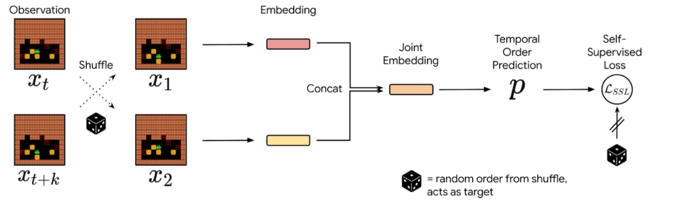 |
| Precedence estimation consists of predicting the temporal order of randomly shuffled events. |
<!–
 |
| Precedence estimation consists of predicting the temporal order of randomly shuffled events. |
 |
| Precedence estimation consists of predicting the temporal order of randomly shuffled events. |
–>
Integrating Reversibility into RL
We propose two concurrent ways of integrating reversibility in RL:
- Reversibility-Aware Exploration (RAE): This approach penalizes irreversible transitions, via a modified reward function. When the agent picks an action that is considered irreversible, it receives a reward corresponding to the environment’s reward minus a positive, fixed penalty, which makes such actions less likely, but does not exclude them.
- Reversibility-Aware Control (RAC): Here, all irreversible actions are filtered out, a process that serves as an intermediate layer between the policy and the environment. When the agent picks an action that is considered irreversible, the action selection process is repeated, until a reversible action is chosen.
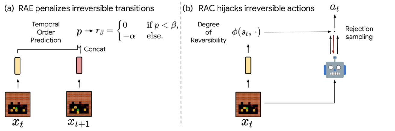 |
| The proposed RAE (left) and RAC (right) methods for reversibility-aware RL. |
<!–
 |
| The proposed RAE (left) and RAC (right) methods for reversibility-aware RL. |
–>
An important distinction between RAE and RAC is that RAE only encourages reversible actions, it does not prohibit them, which means that irreversible actions can still be performed when the benefits outweigh costs (as in the Sokoban example below). As a result, RAC is better suited for safe RL where irreversible side-effects induce risks that should be avoided entirely, and RAE is better suited for tasks where it is suspected that irreversible actions are to be avoided most of the time.
To illustrate the distinction between RAE and RAC, we evaluate the capabilities of both proposed methods. A few example scenarios follow:
- Avoiding (but not prohibiting) irreversible side-effects
A general rule for safe RL is to minimize irreversible interactions when possible, as a principle of caution. To test such capabilities, we introduce a synthetic environment where an agent in an open field is tasked with reaching a goal. If the agent follows the established pathway, the environment remains unchanged, but if it departs from the pathway and onto the grass, the path it takes turns to brown. While this changes the environment, no penalty is issued for such behavior.
In this scenario, a typical model-free agent, such as a Proximal Policy Optimization (PPO) agent, tends to follow the shortest path on average and spoils some of the grass, whereas a PPO+RAE agent avoids all irreversible side-effects.
Top-left: The synthetic environment in which the agent (blue) is tasked with reaching a goal (pink). A pathway is shown in grey leading from the agent to the goal, but it does not follow the most direct route between the two. Top-right: An action sequence with irreversible side-effects of an agent’s actions. When the agent departs from the path, it leaves a brown path through the field. Bottom-left: The visitation heatmap for a PPO agent. Agents tend to follow a more direct path than that shown in grey. Bottom-right: The visitation heatmap for a PPO+RAE agent. The irreversibility of going off-path encourages the agent to stay on the established grey path. - Safe interactions by prohibiting irreversibility
We also tested against the classic Cartpole task, in which the agent controls a cart in order to balance a pole standing precariously upright on top of it. We set the maximum number of interactions to 50k steps, instead of the usual 200. On this task, irreversible actions tend to cause the pole to fall, so it is better to avoid such actions at all.
We show that combining RAC with any RL agent (even a random agent) never fails, given that we select an appropriate threshold for the probability that an action is irreversible. Thus, RAC can guarantee safe, reversible interactions from the very first step in the environment.
We show how the Cartpole performance of a random policy equipped with RAC evolves with different threshold values (ꞵ). Standard model-free agents (DQN, M-DQN) typically score less than 3000, compared to 50000 (the maximum score) for an agent governed by a random+RAC policy at a threshold value of β=0.4. - Avoiding deadlocks in Sokoban
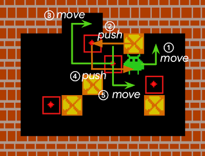
Sokoban is a puzzle game in which the player controls a warehouse keeper and has to push boxes onto target spaces, while avoiding unrecoverable situations (e.g., when a box is in a corner or, in some cases, along a wall).
An action sequence that completes a Sokoban level. Boxes (yellow squares with a red “x”) must be pushed by an agent onto targets (red outlines with a dot in the middle). Because the agent cannot pull the boxes, any box pushed against a wall can be difficult, if not impossible to get away from the wall, i.e., it becomes “deadlocked”. For a standard RL model, early iterations of the agent typically act in a near-random fashion to explore the environment, and consequently, get stuck very often. Such RL agents either fail to solve Sokoban puzzles, or are quite inefficient at it.
Agents that explore randomly quickly engage themselves in deadlocks that prevent them from completing levels (as an example here, pushing the rightmost box on the wall cannot be reversed). We compared the performance in the Sokoban environment of IMPALA, a state-of-the-art model-free RL agent, to that of an IMPALA+RAE agent. We find that the agent with the combined IMPALA+RAE policy is deadlocked less frequently, resulting in superior scores.
The scores of IMPALA and IMPALA+RAE on a set of 1000 Sokoban levels. A new level is sampled at the beginning of each episode.The best score is level dependent and close to 10. In this task, detecting irreversible actions is difficult because it is a highly imbalanced learning problem — only ~1% of actions are indeed irreversible, and many other actions are difficult to flag as reversible, because they can only be reversed through a number of additional steps by the agent.
Reversing an action is sometimes non-trivial. In the example shown here, a box has been pushed against the wall, but is still reversible. However, reversing the situation takes at least five separate movements comprising 17 distinct actions by the agent (each numbered move being the result of several actions from the agent). We estimate that approximately half of all Sokoban levels require at least one irreversible action to be completed (e.g., because at least one target destination is adjacent to a wall). Since IMPALA+RAE solves virtually all levels, it implies that RAE does not prevent the agent from taking irreversible actions when it is crucial to do so.


Conclusion
We present a method that enables RL agents to predict the reversibility of an action by learning to model the temporal order of randomly sampled trajectory events, which results in better exploration and control. Our proposed method is self-supervised, meaning that it does not necessitate any prior knowledge about the reversibility of actions, making it well suited to a variety of environments. In the future, we are interested in studying further how these ideas could be applied in larger scale and safety-critical applications.
Acknowledgements
We would like to thank our paper co-authors Nathan Grinsztajn, Philippe Preux, Olivier Pietquin and Matthieu Geist. We would also like to thank Bobak Shahriari, Théophane Weber, Damien Vincent, Alexis Jacq, Robert Dadashi, Léonard Hussenot, Nino Vieillard, Lukasz Stafiniak, Nikola Momchev, Sabela Ramos and all those who provided helpful discussion and feedback on this work.
Categories
Another Step Towards Breakeven Fusion
For more than 70 years, plasma physicists have dreamed of controlled “breakeven” fusion, where a system is capable of releasing more energy in a fusion reaction than it takes to initiate and sustain those reactions. The challenge is that the reactor must create a plasma at a temperature of tens of millions of degrees, which requires a highly complex, finely tuned system to confine and sustain. Further, creating the plasma and maintaining it, requires substantial amounts of energy, which, to date, have exceeded that released in the fusion reaction itself. Nevertheless, if a “breakeven” system could be achieved, it could provide ample zero-carbon electricity, the potential impact of which has driven interest by government laboratories, such as ITER and the National Ignition Facility, as well as several privately funded efforts.
Today we highlight two recently published papers arising from our collaboration with TAE Technologies1, which demonstrate exciting advancements in the field. In “Overview of C-2W: High-temperature, steady-state beam-driven field-reversed configuration plasmas,” published in Nuclear Fusion, we describe the experimental program implemented by TAE, which leverages our improved version of the Optometrist Algorithm for machine optimization. Due in part to this contribution, the current state-of-the-art reactor is able to achieve plasma lifetimes up to three times longer than its predecessor. In “Multi-instrument Bayesian reconstruction of plasma shape evolution in the C-2W experiment,” published in Physics of Plasmas, we detail new methods developed for analyzing indirect measurements of plasma to reconstruct its properties in detail. This work enabled us to better understand how instabilities in the plasma arise and to understand how to mitigate these perturbations in practice.
Optimizing the Next Generation Fusion Device
The C-2W “Norman” machine (named for TAE’s late co-founder Prof. Norman Rostoker) is a nearly complete rebuild of the C-2U machine that we described in 2017. For this updated version, the TAE team integrated new pressure vessels, new power supplies, a new vacuum system, along with other substantial upgrades.
Norman is incredibly complex, with over 1000 machine control parameters, and likewise, it captures extensive amounts of data for each run, including over 1000 measurements of conditions in the plasma alone. And while the measurements of each plasma experiment are extremely rich, there is no simple metric for “goodness”. Further complicating matters, it is not possible to rapidly iterate to improve performance, because only one experiment can be executed every eight minutes. For these reasons, tuning the system is quite difficult and relies on the expert intuition developed by the plasma physicists operating the system. To optimize the new reactor’s performance, we needed a control system capable of handling the tremendous complexity of the system while being able to quickly tune the control parameters in response to the extensive data generated in experiments.
To accomplish this, we further adapted the Optometrist Algorithm that we had developed for the C-2U system to leverage the expertise of the operators. In this algorithm, the physicists compare experiment pairs, and determine whether the trial better achieves the current goals of the experiment, according to their judgment, than the current reference experiment — e.g., achieving increased plasma size at a fixed temperature, increased temperature, etc. By updating the reference accordingly, machine performance improves over time. However, accounting for operator intuition during this process is critical, because the measure of improvement may not be immediately obvious. For example, under some situations, an experiment with much denser plasma that is a little bit colder may, in fact, be “better”, because it may lead to other improvements in subsequent experiments. We further modified the algorithm by fitting a logistic regression to the binary decisions of the expert to guide the trial experiments, making a classic exploration-exploitation tradeoff.
Applying the Optometrist Algorithm to the magnetic field coils that form the plasma, we found a novel timing sequence that provides consistent starting conditions for long-lived plasmas, almost tripling the plasma lifetime when first applied. This was a marked improvement over the regime of net plasma heating first seen on the C-2U machine in 2015.
 |
| Plasma formation section of the Norman reactor. The outer coils operate for the duration of the experiments while the inner coils accelerate the plasma in less than 10 microseconds. (Photograph by Erik Lucero) |
Bayesian Reconstruction of Plasma Conditions
In addition to optimizing the performance of the machine, we also sought to more thoroughly understand the behavior of the plasmas it is generating. This includes understanding the density profiles, separate electron and ion temperatures, and magnetic fields generated by the plasma. Because the plasma in a fusion generator reaches 30 million Kelvin, which would destroy most solid materials in moments, precise measurements of the plasma conditions are very difficult.
To address this, Norman has a set of indirect diagnostics, generating 5 GB of data per shot, that peer into the plasma without touching it. One of these is a two-story laser interferometer that measures the line-integrated electron density along 14 lines of sight through the plasma, with a sample rate of more than a megahertz. The resulting dataset of line-integrated densities can be used to extract the spatial density profile of the plasma, which is crucial to understanding the plasma behavior. In this case, the Norman reactor generates field-reversed configuration (FRC) plasmas that tend to be best confined when they are hollow (imagine a smoke ring elongated into a barrel shape). The challenge in this situation is that generating the spatial density profiles for such a plasma configuration is an inverse problem, i.e., it is more difficult to infer the shape of the plasma from the measurements (the “inverse” direction) than to predict the measurements from a known shape (the “forward” direction).
 |
| Schematic of C-2W confinement vessel showing measurement systems: interferometer lines of sight measuring electron density (magenta), neutral particle beam lines of sight measuring ion density (purple) and magnetic sensors (blue). These disparate measurements are combined in the Bayesian framework. |
We developed a TensorFlow implementation of the Hamiltonian Monte Carlo (HMC) algorithm to address the problem of inferring the density profile of the plasma from multiple indirect measurements. Because the plasma is described by hundreds to thousands of variables and we want to reconstruct the state for thousands of frames, linked into “bursts” or short movies, for each plasma experiment, processing on CPUs is insufficient. For this reason, we optimized the HMC algorithm to be executed on GPUs. The Bayesian framework for this involves building “forward” models (i.e., predicting effects from causes) for several instruments, which can predict what the instrument would record, given some specified plasma conditions. We can then use HMC to calculate the probabilities of various possible plasma conditions. Understanding both density and temperature are crucial to the problem of breakeven fusion.
High Frequency Plasma Perturbations
Reconstruction of the plasma conditions does more than just recover the plasma density profile, it also recovers the behavior of high frequency density perturbations in the plasma. TAE has done a large number of experiments to determine if Norman’s neutral particle beams and electrode currents can control these oscillations. In the second paper, we demonstrate the strong mitigating effects of the neutral beams, showing that when the neutral beams are turned off, fluctuations immediately begin growing. The reconstruction allows us to see how the radial density profile of the plasma evolves as the perturbations grow, an understanding of which is key to mitigating such perturbations, allowing long-lived stable plasmas. Following a long tradition of listening to plasma perturbations to better intuit their behavior (e.g., ionospheric “whistlers” have been captured by radio operators for over a century), we translate the perturbations to audio (slowed down 500x) in order to listen to them.
| Movie showing spectrogram of magnetic oscillations, played as audio 500 times slower. Different colors indicate different shapes. There is a whistle as the plasma forms, as well as low drum sounds followed immediately by chirps when the plasma destabilizes and recovers. Headphones / earbuds recommended; may annoy pets and humans. |
The Future Looks Hot and Stable
With our assistance using machine optimization and data science, TAE achieved their major goals for Norman, which brings us a step closer to the goal of breakeven fusion. The machine maintains a stable plasma at 30 million Kelvin for 30 milliseconds, which is the extent of available power to its systems. They have completed a design for an even more powerful machine, which they hope will demonstrate the conditions necessary for breakeven fusion before the end of the decade. TAE has succeeded with two complete machine builds during our collaboration, and we are really excited to see the third.
Acknowledgments
We wish to thank Michael Dikovsky, Ian Langmore, Peter Norgaard, Scott Geraedts, Rob von Behren, Bill Heavlin, Anton Kast, Tom Madams, John Platt, Ross Koningstein, and Matt Trevithick for their contributions to this work. We thank the TensorFlow Probability team for considerable implementation assistance. Furthermore, we thank Jeff Dean for visiting TAE’s facility in Southern California and providing thoughtful suggestions. As always we are grateful to our colleagues at TAE Technologies for the opportunity to work on such a fascinating and important problem.
1Google owns stock and warrants in TAE Technologies. ↩
This fall Pixel 6 phones launched with Google Tensor, Google’s first mobile system-on-chip (SoC), bringing together various processing components (such as central/graphic/tensor processing units, image processors, etc.) onto a single chip, custom-built to deliver state-of-the-art innovations in machine learning (ML) to Pixel users. In fact, every aspect of Google Tensor was designed and optimized to run Google’s ML models, in alignment with our AI Principles. That starts with the custom-made TPU integrated in Google Tensor that allows us to fulfill our vision of what should be possible on a Pixel phone.
Today, we share the improvements in on-device machine learning made possible by designing the ML models for Google Tensor’s TPU. We use neural architecture search (NAS) to automate the process of designing ML models, which incentivize the search algorithms to discover models that achieve higher quality while meeting latency and power requirements. This automation also allows us to scale the development of models for various on-device tasks. We’re making these models publicly available through the TensorFlow model garden and TensorFlow Hub so that researchers and developers can bootstrap further use case development on Pixel 6. Moreover, we have applied the same techniques to build a highly energy-efficient face detection model that is foundational to many Pixel 6 camera features.
 |
| An illustration of NAS to find TPU-optimized models. Each column represents a stage in the neural network, with dots indicating different options, and each color representing a different type of building block. A path from inputs (e.g., an image) to outputs (e.g., per-pixel label predictions) through the matrix represents a candidate neural network. In each iteration of the search, a neural network is formed using the blocks chosen at every stage, and the search algorithm aims to find neural networks that jointly minimize TPU latency and/or energy and maximize accuracy. |
Search Space Design for Vision Models
A key component of NAS is the design of the search space from which the candidate networks are sampled. We customize the search space to include neural network building blocks that run efficiently on the Google Tensor TPU.
One widely-used building block in neural networks for various on-device vision tasks is the Inverted Bottleneck (IBN). The IBN block has several variants, each with different tradeoffs, and is built using regular convolution and depthwise convolution layers. While IBNs with depthwise convolution have been conventionally used in mobile vision models due to their low computational complexity, fused-IBNs, wherein depthwise convolution is replaced by a regular convolution, have been shown to improve the accuracy and latency of image classification and object detection models on TPU.
However, fused-IBNs can have prohibitively high computational and memory requirements for neural network layer shapes that are typical in the later stages of vision models, limiting their use throughout the model and leaving the depthwise-IBN as the only alternative. To overcome this limitation, we introduce IBNs that use group convolutions to enhance the flexibility in model design. While regular convolution mixes information across all the features in the input, group convolution slices the features into smaller groups and performs regular convolution on features within that group, reducing the overall computational cost. Called group convolution–based IBNs (GC-IBNs), their tradeoff is that they may adversely impact model quality.
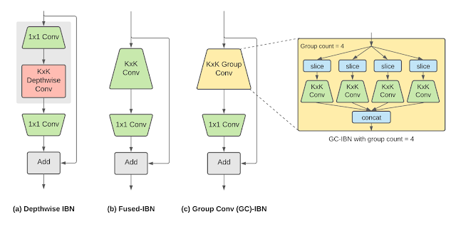 |
| Inverted bottleneck (IBN) variants: (a) depthwise-IBN, depthwise convolution layer with filter size KxK sandwiched between two convolution layers with filter size 1×1; (b) fused-IBN, convolution and depthwise are fused into a convolution layer with filter size KxK; and (c) group convolution–based GC-IBN that replaces with the KxK regular convolution in fused-IBN with group convolution. The number of groups (group count) is a tunable parameter during NAS. |
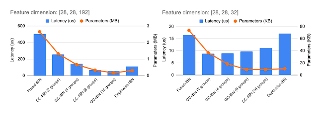 |
| Inclusion of GC-IBN as an option provides additional flexibility beyond other IBNs. Computational cost and latency of different IBN variants depends on the feature dimensions being processed (shown above for two example feature dimensions). We use NAS to determine the optimal choice of IBN variants. |
Faster, More Accurate Image Classification
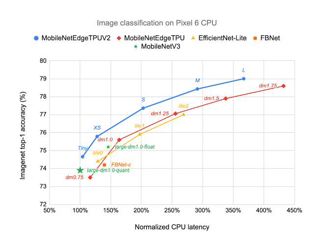
Which IBN variant to use at which stage of a deep neural network depends on the latency on the target hardware and the performance of the resulting neural network on the given task. We construct a search space that includes all of these different IBN variants and use NAS to discover neural networks for the image classification task that optimize the classification accuracy at a desired latency on TPU. The resulting MobileNetEdgeTPUV2 model family improves the accuracy at a given latency (or latency at a desired accuracy) compared to the existing on-device models when run on the TPU. MobileNetEdgeTPUV2 also outperforms their predecessor, MobileNetEdgeTPU, the image classification models designed for the previous generation of the TPU.
 |
| Network architecture families visualized as connected dots at different latency targets. Compared with other mobile models, such as FBNet, MobileNetV3, and EfficientNets, MobileNetEdgeTPUV2 models achieve higher ImageNet top-1 accuracy at lower latency when running on Google Tensor’s TPU. |
MobileNetEdgeTPUV2 models are built using blocks that also improve the latency/accuracy tradeoff on other compute elements in the Google Tensor SoC, such as the CPU. Unlike accelerators such as the TPU, CPUs show a stronger correlation between the number of multiply-and-accumulate operations in the neural network and latency. GC-IBNs tend to have fewer multiply-and-accumulate operations than fused-IBNs, which leads MobileNetEdgeTPUV2 to outperform other models even on Pixel 6 CPU.
 |
| MobileNetEdgeTPUV2 models achieve ImageNet top-1 accuracy at lower latency on Pixel 6 CPU, and outperform other CPU-optimized model architectures, such as MobileNetV3. |
Improving On-Device Semantic Segmentation
Many vision models consist of two components, the base feature extractor for understanding general features of the image, and the head for understanding domain-specific features, such as semantic segmentation (the task of assigning labels, such as sky, car, etc., to each pixel in an image) and object detection (the task of detecting instances of objects, such as cats, doors, cars, etc., in an image). Image classification models are often used as feature extractors for these vision tasks. As shown below, the MobileNetEdgeTPUV2 classification model coupled with the DeepLabv3+ segmentation head improves the quality of on-device segmentation.
To further improve the segmentation model quality, we use the bidirectional feature pyramid network (BiFPN) as the segmentation head, which performs weighted fusion of different features extracted by the feature extractor. Using NAS we find the optimal configuration of blocks in both the feature extractor and the BiFPN head. The resulting models, named Autoseg-EdgeTPU, produce even higher-quality segmentation results, while also running faster.
The final layers of the segmentation model contribute significantly to the overall latency, mainly due to the operations involved in generating a high resolution segmentation map. To optimize the latency on TPU, we introduce an approximate method for generating the high resolution segmentation map that reduces the memory requirement and provides a nearly 1.5x speedup, without significantly impacting the segmentation quality.
 |
| Left: Comparing the performance, measured as mean intersection-over-union (mIOU), of different segmentation models on the ADE20K semantic segmentation dataset (top 31 classes). Right: Approximate feature upsampling (e.g., increasing resolution from 32×32 → 512×512). Argmax operation used to compute per-pixel labels is fused with the bilinear upsampling. Argmax performed on smaller resolution features reduces memory requirements and improves latency on TPU without a significant impact to quality. |
Higher-Quality, Low-Energy Object Detection
Classic object detection architectures allocate ~70% of the compute budget to the feature extractor and only ~30% to the detection head. For this task we incorporate the GC-IBN blocks into a search space we call “Spaghetti Search Space”1, which provides the flexibility to move more of the compute budget to the head. This search space also uses the non-trivial connection patterns seen in recent NAS works such as MnasFPN to merge different but related stages of the network to strengthen understanding.
We compare the models produced by NAS to MobileDet-EdgeTPU, a class of mobile detection models customized for the previous generation of TPU. MobileDets have been demonstrated to achieve state-of-the-art detection quality on a variety of mobile accelerators: DSPs, GPUs, and the previous TPU. Compared with MobileDets, the new family of SpaghettiNet-EdgeTPU detection models achieves +2.2% mAP (absolute) on COCO at the same latency and consumes less than 70% of the energy used by MobileDet-EdgeTPU to achieve similar accuracy.
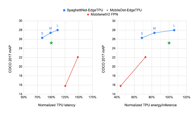 |
| Comparing the performance of different object detection models on the COCO dataset with the mAP metric (higher is better). SpaghettiNet-EdgeTPU achieves higher detection quality at lower latency and energy consumption compared to previous mobile models, such as MobileDets and MobileNetV2 with Feature Pyramid Network (FPN). |
Inclusive, Energy-Efficient Face Detection
Face detection is a foundational technology in cameras that enables a suite of additional features, such as fixing the focus, exposure and white balance, and even removing blur from the face with the new Face Unblur feature. Such features must be designed responsibly, and Face Detection in the Pixel 6 were developed with our AI Principles top of mind.
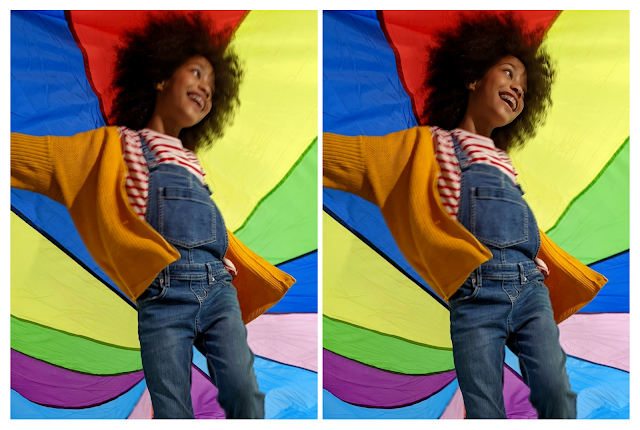 |
| Left: The original photo without improvements. Right: An unblurred face in a dynamic environment. This is the result of Face Unblur combined with a more accurate face detector running at a higher frames per second. |
Since mobile cameras can be power-intensive, it was important for the face detection model to fit within a power budget. To optimize for energy efficiency, we used the Spaghetti Search Space with an algorithm to search for architectures that maximize accuracy at a given energy target. Compared with a heavily optimized baseline model, SpaghettiNet achieves the same accuracy at ~70% of the energy. The resulting face detection model, called FaceSSD, is more power-efficient and accurate. This improved model, combined with our auto-white balance and auto-exposure tuning improvements, are part of Real Tone on Pixel 6. These improvements help better reflect the beauty of all skin tones. Developers can utilize this model in their own apps through the Android Camera2 API.
Toward Datacenter-Quality Language Models on a Mobile Device
Deploying low-latency, high-quality language models on mobile devices benefits ML tasks like language understanding, speech recognition, and machine translation. MobileBERT, a derivative of BERT, is a natural language processing (NLP) model tuned for mobile CPUs.
However, due to the various architectural optimizations made to run these models efficiently on mobile CPUs, their quality is not as high as that of the large BERT models. Since MobileBERT on TPU runs significantly faster than on CPU, it presents an opportunity to improve the model architecture further and reduce the quality gap between MobileBERT and BERT. We extended the MobileBERT architecture and leveraged NAS to discover models that map well to the TPU. These new variants of MobileBERT, named MobileBERT-EdgeTPU, achieve up to 2x higher hardware utilization, allowing us to deploy large and more accurate models on TPU at latencies comparable to the baseline MobileBERT.
MobileBERT-EdgeTPU models, when deployed on Google Tensor’s TPU, produce on-device quality comparable to the large BERT models typically deployed in data centers.
 |
| Performance on the question answering task (SQuAD v 1.1). While the TPU in Pixel 6 provides a ~10x acceleration over CPU, further model customization for the TPU achieves on-device quality comparable to the large BERT models typically deployed in data centers. |
Conclusion
In this post, we demonstrated how designing ML models for the target hardware expands the on-device ML capabilities of Pixel 6 and brings high-quality, ML-powered experiences to Pixel users. With NAS, we scaled the design of ML models to a variety of on-device tasks and built models that provide state-of-the-art quality on-device within the latency and power constraints of a mobile device. Researchers and ML developers can try out these models in their own use cases by accessing them through the TensorFlow model garden and TF Hub.
Acknowledgements
This work is made possible through a collaboration spanning several teams across Google. We’d like to acknowledge contributions from Rachit Agrawal, Berkin Akin, Andrey Ayupov, Aseem Bathla, Gabriel Bender, Po-Hsein Chu, Yicheng Fan, Max Gubin, Jaeyoun Kim, Quoc Le, Dongdong Li, Jing Li, Yun Long, Hanxiao Lu, Ravi Narayanaswami, Benjamin Panning, Anton Spiridonov, Anakin Tung, Zhuo Wang, Dong Hyuk Woo, Hao Xu, Jiayu Ye, Hongkun Yu, Ping Zhou, and Yanqi Zhuo. Finally, we’d like to thank Tom Small for creating illustrations for this blog post.
1The resulting architectures tend to look like spaghetti because of the connection patterns formed between blocks. ↩
Categories
Google at EMNLP 2021
This week, the annual conference on Empirical Methods in Natural Language Processing (EMNLP 2021) will be held both virtually and in Punta Cana, Dominican Republic. As a Diamond Level sponsor of EMNLP 2021, Google will contribute research on a diverse set of topics, including language interactions, causal inference, and question answering, additionally serving in various levels of organization in the conference.
Below is a full list of Google’s involvement and publications being presented at EMNLP 2021. We congratulate these authors, and all other researchers who are presenting their work at the conference (Google affiliations presented in bold).
Organizing Committee
Ethics Committee includes: Nyalleng Moorosi
Publications
MATE: Multi-view Attention for Table Transformer Efficiency (see blog post)
Julian Martin Eisenschlos, Maharshi Gor*, Thomas Müller*, William W. Cohen
Residual Adapters for Parameter-Efficient ASR Adaptation to Atypical and Accented Speech (see blog post)
Katrin Tomanek, Vicky Zayats, Dirk Padfield, Kara Vaillancourt, Fadi Biadsy
Towards Automatic Evaluation of Dialog Systems: A Model-Free Off-Policy Evaluation Approach (see blog post)
Haoming Jiang*, Bo Dai, Mengjiao Yang,Tuo Zhao, Wei Wei
Case-Based Reasoning for Natural Language Queries Over Knowledge Bases
Rajarshi Das, Manzil Zaheer, Dung Thai, Ameya Godbole, Ethan Perez, Jay-Yoon Lee, Lizhen Tan, Lazaros Polymenakos, Andrew McCallum
XTREME-R: Towards More Challenging and Nuanced Multilingual Evaluation (see blog post)
Sebastian Ruder, Noah Constant, Jan Botha, Aditya Siddhant, Orhan Firat, Jinlan Fu, Pengfei Liu, Junjie Hu, Dan Garrette, Graham Neubig, Melvin Johnson
Building and Evaluating Open-Domain Dialogue Corpora with Clarifying Questions
Mohammad Aliannejadi, Julia Kiseleva, Aleksandr Chuklin, Jeffrey Dalton, Mikhail Burtsev
Fast WordPiece Tokenization
Xinying Song, Alex Salcianu, Yang Song*, Dave Dopson, Denny Zhou
Frequency Effects on Syntactic Rule Learning in Transformers
Jason Wei, Dan Garrette, Tal Linzen, Ellie Pavlick
Controllable Semantic Parsing via Retrieval Augmentation
Panupong Pasupat, Yuan Zhang, Kelvin Guu
Systematic Generalization on gSCAN: What is Nearly Solved and What is Next?
Linlu Qiu*, Hexiang Hu,Bowen Zhang, Peter Shaw, Fei Sha
Effective Sequence-to-Sequence Dialogue State Tracking
Jeffrey Zhao, Mahdis Mahdieh, Ye Zhang, Yuan Cao, Yonghui Wu
Learning Compact Metrics for MT
Amy Pu*, Hyung Won Chung*, Ankur P. Parikh, Sebastian Gehrmann, Thibault Sellam
Joint Passage Ranking for Diverse Multi-answer Retrieval
Sewon Min*, Kenton Lee, Ming-Wei Chang, Kristina Toutanova, Hannaneh Hajishirzi
Toward Deconfounding the Effect of Entity Demographics for Question Answering Accuracy
Maharshi Gor*, Kellie Webster, Jordan Boyd-Graber*
Good-Enough Example Extrapolation
Jason Wei
Q2: Evaluating Factual Consistency in Knowledge-Grounded Dialogues via Question Generation and Question Answering
Or Honovich*, Leshem Choshen, Roee Aharoni, Ella Neeman, Idan Szpektor, Omri Abend
The Power of Scale for Parameter-Efficient Prompt Tuning
Brian Lester*, Rami Al-Rfou, Noah Constant
A Simple and Effective Method to Eliminate the Self Language Bias in Multilingual Representations
Ziyi Yang*, Yinfei Yang, Daniel Cer, Eric Darve
Universal Sentence Representation Learning with Conditional Masked Language Model
Ziyi Yang*, Yinfei Yang, Daniel Cer, Jax Law, Eric Darve
Scalable Font Reconstruction with Dual Latent Manifolds
Nikita Srivatsan, Si Wu, Jonathan T. Barron, Taylor Berg-Kirkpatrick
Structured Context and High-Coverage Grammar for Conversational Question Answering Over Knowledge Graphs
Pierre Marion, Paweł Krzysztof Nowak, Francesco Piccinno
Don’t Search for a Search Method — Simple Heuristics Suffice for Adversarial Text Attacks
Nathaniel Berger*, Stefan Riezler, Artem Sokolov, Sebastian Ebert
HintedBT: Augmenting Back-Translation with Quality and Transliteration Hints
Sahana Ramnath, Melvin Johnson, Abhirut Gupta, Aravindan Raghuveer
STraTA: Self-Training with Task Augmentation for Better Few-Shot Learning
Tu Vu*, Minh-Thang Luong, Quoc V. Le, Grady Simon,Mohit Iyyer
Do Transformer Modifications Transfer Across Implementations and Applications? (See blog post)
Sharan Narang, Hyung Won Chung, Yi Tay, William Fedus, Thibault Fevry*, Michael Matena*, Karishma Malkan*, Noah Fiedel, Noam Shazeer, Zhenzhong Lan*, Yanqi Zhou, Wei Li, Nan Ding, Jake Marcus, Adam Roberts, Colin Raffel*
A Large-Scale Study of Machine Translation in Turkic Languages
Jamshidbek Mirzakhalova, Anoop Babua, Duygu Atamana, Sherzod Karieva, Francis Tyersa, Otabek Abduraufova, Mammad Hajilia, Sardana Ivanovaa, Abror Khaytbaeva, Antonio Laverghetta Jr., Behzodbek Moydinboyeva, Esra Onala, Shaxnoza Pulatovaa, Ahsan Wahaba, Orhan Firat, Sriram Chellappan
ReasonBERT: Pre-trained to Reason with Distant Supervision
Xiang Deng, Yu Su, Alyssa Lees, You Wu, Cong Yu, Huan Sun
MasakhaNER: Named Entity Recognition for African Languages
David Ifeoluwa Adelani, Jade Abbott, Graham Neubig, Daniel D’souza, Julia Kreutzer, Constantine Lignos, Chester Palen-Michel, Happy Buzaaba, Shruti Rijhwani, Sebastian Ruder, Stephen Mayhew, Israel Abebe Azime, Shamsuddeen H. Muhammad, Chris Chinenye Emezue, Joyce Nakatumba-Nabende, Perez Ogayo, Anuoluwapo Aremu, Catherine Gitau, Derguene Mbaye, Jesujoba Alabi, Seid Muhie Yimam, Tajuddeen Rabiu Gwadabe, Ignatius Ezeani, Rubungo Andre Niyongabo, Jonathan Mukiibi, Verrah Otiende, Iroro Orife, Davis David, Samba Ngom, Tosin Adewumi, Paul Rayson, Mofetoluwa Adeyemi, Gerald Muriuki, Emmanuel Anebi, Chiamaka Chukwuneke, Nkiruka Odu, Eric Peter Wairagala, Samuel Oyerinde, Clemencia Siro, Tobius Saul Bateesa, Temilola Oloyede, Yvonne Wambui, Victor Akinode, Deborah Nabagereka, Maurice Katusiime, Ayodele Awokoya, Mouhamadane MBOUP, Dibora Gebreyohannes, Henok Tilaye, Kelechi Nwaike, Degaga Wolde, Abdoulaye Faye, Blessing Sibanda, Orevaoghene Ahia, Bonaventure F. P. Dossou, Kelechi Ogueji, Thierno Ibrahima DIOP, Abdoulaye Diallo, Adewale Akinfaderin, Tendai Marengereke, Salomey Osei
Multi-stage Training with Improved Negative Contrast for Neural Passage Retrieval
Jing Lu*, Gustavo Hernandez, Abrego, Ji Ma, Jianmo Ni, Yinfei Yang
Controlling Machine Translation for Multiple Attributes with Additive Interventions
Andrea Schioppa, Artem Sokolov, David Vilar, Katja Filippova
A Simple and Effective Positional Encoding for Transformers
Pu-Chin Chen, Henry Tsai, Srinadh Bhojanapalli, Hyung Won Chung, Yin-Wen Chang, Chun-Sung Ferng
CrossVQA: Scalably Generating Benchmarks for Systematically Testing VQA Generalization
Arjun R. Akula*, Soravit Changpinyo, Boqing Gong, Piyush Sharma, Song-Chun Zhu, Radu Soricut
Can We Improve Model Robustness through Secondary Attribute Counterfactuals?
Ananth Balashankar, Xuezhi Wang, Ben Packer, Nithum Thain, Ed Chi, Alex Beutel
Multi-Vector Attention Models for Deep Re-ranking
Giulio Zhou*, Jacob Devlin
Diverse Distributions of Self-Supervised Tasks for Meta-Learning in NLP
Trapit Bansal, Karthick Gunasekaran, Tong Wang, Tsendsuren Munkhdalai, Andrew McCallum
Workshops
NLP for Conversational AI
Invited speakers include: Idan Szpektor
Organizers include: Abhinav Rastogi
Novel Ideas in Learning-to-Learn Through Interaction
Invited speakers include: Natasha Jaques
Evaluation & Comparison of NLP Systems
Invited speakers include: Sebastian Ruder
Causal Inference & NLP
Organizers include: Amir Feder, Jacob Eisenstein, Victor Veitch
Machine Reading for Question Answering
Invited speakers include: Jon Clark
Computational Approaches to Discourse
Organizers include: Annie Louis
New Frontiers in Summarization
Invited speakers include: Sebastian Gehrmann, Shashi Narayan
Multi-lingual Representation Learning
Invited speakers include: Melvin Johnson
Organizers include: Alexis Conneau, Orhan Firat, Sebastian Ruder
Widening in NLP
Invited speakers include: Jasmijn Bastings
Organizers include: Shaily Bhatt
Evaluations and Assessments of Neural Conversation Systems (EANCS)
Organizers include: Wei Wei, Bo Dai
BlackboxNLP
Invited speakers include: Sara Hooker
Organizers include: Jasmijn Bastings
Tutorials
Multi-Domain Multilingual Question Answering
Organizers include: Sebastian Ruder
Demos
LMdiff: A Visual Diff Tool to Compare Language Models
Hendrik Strobelt, Benjamin Hoover, Arvind Satyanarayan, Sebastian Gehrmann
*Work done while at Google. ↩
Categories
Enhanced Sleep Sensing in Nest Hub
Earlier this year, we launched Contactless Sleep Sensing in Nest Hub, an opt-in feature that can help users better understand their sleep patterns and nighttime wellness. While some of the most critical sleep insights can be derived from a person’s overall schedule and duration of sleep, that alone does not tell the complete story. The human brain has special neurocircuitry to coordinate sleep cycles — transitions between deep, light, and rapid eye movement (REM) stages of sleep — vital not only for physical and emotional wellbeing, but also for optimal physical and cognitive performance. Combining such sleep staging information with disturbance events can help you better understand what’s happening while you’re sleeping.
Today we announced enhancements to Sleep Sensing that provide deeper sleep insights. While not intended for medical purposes1, these enhancements allow better understanding of sleep through sleep stages and the separation of the user’s coughs and snores from other sounds in the room. Here we describe how we developed these novel technologies, through transfer learning techniques to estimate sleep stages and sensor fusion of radar and microphone signals to disambiguate the source of sleep disturbances.
 |
| To help people understand their sleep patterns, Nest Hub displays a hypnogram, plotting the user’s sleep stages over the course of a sleep session. Potential sound disturbances during sleep will now include “Other sounds” in the timeline to separate the user’s coughs and snores from other sound disturbances detected from sources in the room outside of the calibrated sleeping area. |
Training and Evaluating the Sleep Staging Classification Model
Most people cycle through sleep stages 4-6 times a night, about every 80-120 minutes, sometimes with a brief awakening between cycles. Recognizing the value for users to understand their sleep stages, we have extended Nest Hub’s sleep-wake algorithms using Soli to distinguish between light, deep, and REM sleep. We employed a design that is generally similar to Nest Hub’s original sleep detection algorithm: sliding windows of raw radar samples are processed to produce spectrogram features, and these are continuously fed into a Tensorflow Lite model. The key difference is that this new model was trained to predict sleep stages rather than simple sleep-wake status, and thus required new data and a more sophisticated training process.
In order to assemble a rich and diverse dataset suitable for training high-performing ML models, we leveraged existing non-radar datasets and applied transfer learning techniques to train the model. The gold standard for identifying sleep stages is polysomnography (PSG), which employs an array of wearable sensors to monitor a number of body functions during sleep, such as brain activity, heartbeat, respiration, eye movement, and motion. These signals can then be interpreted by trained sleep technologists to determine sleep stages.
To develop our model, we used publicly available data from the Sleep Heart Health Study (SHHS) and Multi-ethnic Study of Atherosclerosis (MESA) studies with over 10,000 sessions of raw PSG sensor data with corresponding sleep staging ground-truth labels, from the National Sleep Research Resource. The thoracic respiratory inductance plethysmography (RIP) sensor data within these PSG datasets is collected through a strap worn around the patient’s chest to measure motion due to breathing. While this is a very different sensing modality from radar, both RIP and radar provide signals that can be used to characterize a participant’s breathing and movement. This similarity between the two domains makes it possible to leverage a plethysmography-based model and adapt it to work with radar.
To do so, we first computed spectrograms from the RIP time series signals and used these as features to train a convolutional neural network (CNN) to predict the groundtruth sleep stages. This model successfully learned to identify breathing and motion patterns in the RIP signal that could be used to distinguish between different sleep stages. This indicated to us that the same should also be possible when using radar-based signals.
To test the generality of this model, we substituted similar spectrogram features computed from Nest Hub’s Soli sensor and evaluated how well the model was able to generalize to a different sensing modality. As expected, the model trained to predict sleep stages from a plethysmograph sensor was much less accurate when given radar sensor data instead. However, the model still performed much better than chance, which demonstrated that it had learned features that were relevant across both domains.
To improve on this, we collected a smaller secondary dataset of radar sensor data with corresponding PSG-based groundtruth labels, and then used a portion of this dataset to fine-tune the weights of the initial model. This smaller amount of additional training data allowed the model to adapt the original features it had learned from plethysmography-based sleep staging and successfully generalize them to our domain. When evaluated on an unseen test set of new radar data, we found the fine-tuned model produced sleep staging results comparable to that of other consumer sleep trackers.
 |
| The custom ML model efficiently processes a continuous stream of 3D radar tensors (as shown in the spectrogram at the top of the figure) to automatically compute probabilities of each sleep stage — REM, light, and deep — or detect if the user is awake or restless. |
More Intelligent Audio Sensing Through Audio Source Separation
Soli-based sleep tracking gives users a convenient and reliable way to see how much sleep they are getting and when sleep disruptions occur. However, to understand and improve their sleep, users also need to understand why their sleep may be disrupted. We’ve previously discussed how Nest Hub can help monitor coughing and snoring, frequent sources of sleep disturbances of which people are often unaware. To provide deeper insight into these disturbances, it is important to understand if the snores and coughs detected are your own.
The original algorithms on Nest Hub used an on-device, CNN-based detector to process Nest Hub’s microphone signal and detect coughing or snoring events, but this audio-only approach did not attempt to distinguish from where a sound originated. Combining audio sensing with Soli-based motion and breathing cues, we updated our algorithms to separate sleep disturbances from the user-specified sleeping area versus other sources in the room. For example, when the primary user is snoring, the snoring in the audio signal will correspond closely with the inhalations and exhalations detected by Nest Hub’s radar sensor. Conversely, when snoring is detected outside the calibrated sleeping area, the two signals will vary independently. When Nest Hub detects coughing or snoring but determines that there is insufficient correlation between the audio and motion features, it will exclude these events from the user’s coughing or snoring timeline and instead note them as “Other sounds” on Nest Hub’s display. The updated model continues to use entirely on-device audio processing with privacy-preserving analysis, with no raw audio data sent to Google’s servers. A user can then opt to save the outputs of the processing (sound occurrences, such as the number of coughs and snore minutes) in Google Fit, in order to view their night time wellness over time.
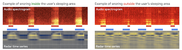 |
| Snoring sounds that are synchronized with the user’s breathing pattern (left) will be displayed in the user’s Nest Hub’s Snoring timeline. Snoring sounds that do not align with the user’s breathing pattern (right) will be displayed in Nest Hub’s “Other sounds” timeline. |
Since Nest Hub with Sleep Sensing launched, researchers have expressed interest in investigational studies using Nest Hub’s digital quantification of nighttime cough. For example, a small feasibility study supported by the Cystic Fibrosis Foundation2 is currently underway to evaluate the feasibility of measuring night time cough using Nest Hub in families of children with cystic fibrosis (CF), a rare inherited disease, which can result in a chronic cough due to mucus in the lungs. Researchers are exploring if quantifying cough at night could be a proxy for monitoring response to treatment.
Conclusion
Based on privacy-preserving radar and audio signals, these improved sleep staging and audio sensing features on Nest Hub provide deeper insights that we hope will help users translate their night time wellness into actionable improvements for their overall wellbeing.
Acknowledgements
This work involved collaborative efforts from a multidisciplinary team of software engineers, researchers, clinicians, and cross-functional contributors. Special thanks to Dr. Logan Schneider, a sleep neurologist whose clinical expertise and contributions were invaluable to continuously guide this research. In addition to the authors, key contributors to this research include Anupam Pathak, Jeffrey Yu, Arno Charton, Jian Cui, Sinan Hersek, Jonathan Hsu, Andi Janti, Linda Lei, Shao-Po Ma, Jo Schaeffer, Neil Smith, Siddhant Swaroop, Bhavana Koka, Dr. Jim Taylor, and the extended team. Thanks to Mark Malhotra and Shwetak Patel for their ongoing leadership, as well as the Nest, Fit, and Assistant teams we collaborated with to build and validate these enhancements to Sleep Sensing on Nest Hub.
1Not intended to diagnose, cure, mitigate, prevent or treat any disease or condition. ↩
2Google did not have any role in study design, execution, or funding. ↩
When building a deep model for a new machine learning application, researchers often begin with existing network architectures, such as ResNets or EfficientNets. If the initial model’s accuracy isn’t high enough, a larger model may be a tempting alternative, but may not actually be the best solution for the task at hand. Instead, better performance potentially could be achieved by designing a new model that is optimized for the task. However, such efforts can be challenging and usually require considerable resources.
In “Wisdom of Committees: An Overlooked Approach to Faster and More Accurate Models”, we discuss model ensembles and a subset called model cascades, both of which are simple approaches that construct new models by collecting existing models and combining their outputs. We demonstrate that ensembles of even a small number of models that are easily constructed can match or exceed the accuracy of state-of-the-art models while being considerably more efficient.
What Are Model Ensembles and Cascades?
Ensembles and cascades are related approaches that leverage the advantages of multiple models to achieve a better solution. Ensembles execute multiple models in parallel and then combine their outputs to make the final prediction. Cascades are a subset of ensembles, but execute the collected models sequentially, and merge the solutions once the prediction has a high enough confidence. For simple inputs, cascades use less computation, but for more complex inputs, may end up calling on a greater number of models, resulting in higher computation costs.
 |
| Overview of ensembles and cascades. While this example shows 2-model combinations for both ensembles and cascades, any number of models can potentially be used. |
Compared to a single model, ensembles can provide improved accuracy if there is variety in the collected models’ predictions. For example, the majority of images in ImageNet are easy for contemporary image recognition models to classify, but there are many images for which predictions vary between models and that will benefit most from an ensemble.
While ensembles are well-known, they are often not considered a core building block of deep model architectures and are rarely explored when researchers are developing more efficient models (with a few notable exceptions [1, 2, 3]). Therefore, we conduct a comprehensive analysis of ensemble efficiency and show that a simple ensemble or cascade of off-the-shelf pre-trained models can enhance both the efficiency and accuracy of state-of-the-art models.
To encourage the adoption of model ensembles, we demonstrate the following beneficial properties:
- Simple to build: Ensembles do not require complicated techniques (e.g., early exit policy learning).
- Easy to maintain: Ensembles are trained independently, making them easy to maintain and deploy.
- Affordable to train: The total training cost of models in an ensemble is often lower than a similarly accurate single model.
- On-device speedup: The reduction in computation cost (FLOPS) successfully translates to a speedup on real hardware.
Efficiency and Training Speed
It’s not surprising that ensembles can increase accuracy, but using multiple models in an ensemble may introduce extra computational cost at runtime. So, we investigate whether an ensemble can be more accurate than a single model that has the same computational cost. We analyze a series of models, EfficientNet-B0 to EfficientNet-B7, that have different levels of accuracy and FLOPS when applied to ImageNet inputs. The ensemble predictions are computed by averaging the predictions of each individual model.
We find that ensembles are significantly more cost-effective in the large computation regime (>5B FLOPS). For example, an ensemble of two EfficientNet-B5 models matches the accuracy of a single EfficientNet-B7 model, but does so using ~50% fewer FLOPS. This demonstrates that instead of using a large model, in this situation, one should use an ensemble of multiple considerably smaller models, which will reduce computation requirements while maintaining accuracy. Moreover, we find that the training cost of an ensemble can be much lower (e.g., two B5 models: 96 TPU days total; one B7 model: 160 TPU days). In practice, model ensemble training can be parallelized using multiple accelerators leading to further reductions. This pattern holds for the ResNet and MobileNet families as well.
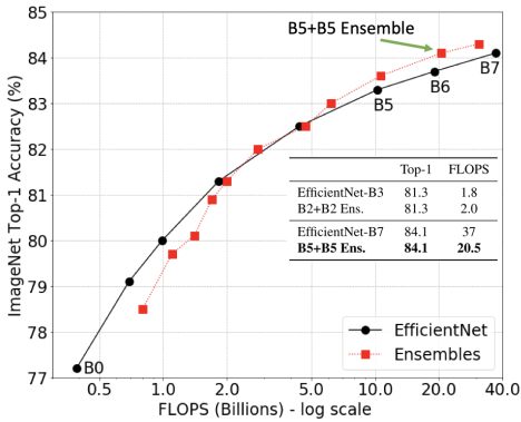 |
| Ensembles outperform single models in the large computation regime (>5B FLOPS). |
Power and Simplicity of Cascades
While we have demonstrated the utility of model ensembles, applying an ensemble is often wasteful for easy inputs where a subset of the ensemble will give the correct answer. In these situations, cascades save computation by allowing for an early exit, potentially stopping and outputting an answer before all models are used. The challenge is to determine when to exit from the cascade.
To highlight the practical benefit of cascades, we intentionally choose a simple heuristic to measure the confidence of the prediction — we take the confidence of the model to be the maximum of the probabilities assigned to each class. For example, if the predicted probabilities for an image being either a cat, dog, or horse were 20%, 80% and 20%, respectively, then the confidence of the model’s prediction (dog) would be 0.8. We use a threshold on the confidence score to determine when to exit from the cascade.
To test this approach, we build model cascades for the EfficientNet, ResNet, and MobileNetV2 families to match either computation costs or accuracy (limiting the cascade to a maximum of four models). By design in cascades, some inputs incur more FLOPS than others, because more challenging inputs go through more models in the cascade than easier inputs. So we report the average FLOPS computed over all test images. We show that cascades outperform single models in all computation regimes (when FLOPS range from 0.15B to 37B) and can enhance accuracy or reduce the FLOPS (sometimes both) for all models tested.
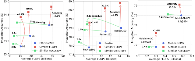 |
| Cascades of EfficientNet (left), ResNet (middle) and MobileNetV2 (right) models on ImageNet. When using similar FLOPS, cascades obtain a higher accuracy than single models (shown by the red arrows pointing up). Cascades can also match the accuracy of single models with significantly fewer FLOPS e.g., 5.4x for B7 (green arrows pointing left). |
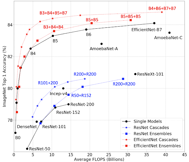 |
| Summary of accuracy vs. FLOPS for ensembles and cascades. Squares and stars represent ensembles and cascades, respectively,, and the “+” notation indicates the models that comprise the ensemble or cascade. For example, ”B3+B4+B5+B7” at a star refers to a cascade of EfficientNet-B3, B4, B5 and B7 models. |
In some cases it is not the average computation cost but the worst-case cost that is the limiting factor. By adding a simple constraint to the cascade building procedure, one can guarantee an upper bound to the computation cost of the cascade. See the paper for more details.
Other than convolutional neural networks, we also consider a Transformer-based architecture, ViT. We build a cascade of ViT-Base and ViT-Large models to match the average computation or accuracy of a single state-of-the-art ViT-Large model, and show that the benefit of cascades also generalizes to Transformer-based architectures.
| Single Models | Cascades – Similar Throughput | Cascades – Similar Accuracy | ||||||
| Top-1 (%) | Throughput | Top-1 (%) | Throughput | △Top-1 | Top-1 (%) | Throughput | SpeedUp | |
| ViT-L-224 | 82.0 | 192 | 83.1 | 221 | 1.1 | 82.3 | 409 | 2.1x |
| ViT-L-384 | 85.0 | 54 | 86.0 | 69 | 1.0 | 85.2 | 125 | 2.3x |
| Cascades of ViT models on ImageNet. “224” and “384” indicate the image resolution on which the model is trained. Throughput is measured as the number of images processed per second. Our cascades can achieve a 1.0% higher accuracy than ViT-L-384 with a similar throughput or achieve a 2.3x speedup over that model while matching its accuracy. |
Earlier works on cascades have also shown efficiency improvements for state-of-the-art models, but here we demonstrate that a simple approach with a handful of models is sufficient.
Inference Latency
In the above analysis, we average FLOPS to measure the computational cost. It is also important to verify that the FLOPS reduction obtained by cascades actually translates into speedup on hardware. We examine this by comparing on-device latency and speed-up for similarly performing single models versus cascades. We find a reduction in the average online latency on TPUv3 of up to 5.5x for cascades of models from the EfficientNet family compared to single models with comparable accuracy. As models become larger the more speed-up we find with comparable cascades.
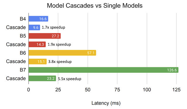 |
| Average latency of cascades on TPUv3 for online processing. Each pair of same colored bars has comparable accuracy. Notice that cascades provide drastic latency reduction. |
Building Cascades from Large Pools of Models
Above, we limit the model types and only consider ensembles/cascades of at most four models. While this highlights the simplicity of using ensembles, it also allows us to check all combinations of models in very little time so we can find optimal model collections with only a few CPU hours on a held out set of predictions.
When a large pool of models exists, we would expect cascades to be even more efficient and accurate, but brute force search is not feasible. However, efficient cascade search methods have been proposed. For example, the algorithm of Streeter (2018), when applied to a large pool of models, produced cascades that matched the accuracy of state-of-the-art neural architecture search–based ImageNet models with significantly fewer FLOPS, for a range of model sizes.
Conclusion
As we have seen, ensemble/cascade-based models obtain superior efficiency and accuracy over state-of-the-art models from several standard architecture families. In our paper we show more results for other models and tasks. For practitioners, this outlines a simple procedure to boost accuracy while retaining efficiency using off-the-shelf models. We encourage you to try it out!
Acknowledgement
This blog presents research done by Xiaofang Wang (while interning at Google Research), Dan Kondratyuk, Eric Christiansen, Kris M. Kitani, Yair Alon (prev. Movshovitz-Attias), and Elad Eban. We thank Sergey Ioffe, Shankar Krishnan, Max Moroz, Josh Dillon, Alex Alemi, Jascha Sohl-Dickstein, Rif A Saurous, and Andrew Helton for their valuable help and feedback.