
 In this round of MLPerf training v1.1, optimization across the entire stack including hardware, system software, libraries, and algorithms continue to boost NVIDIA MLPerf training performance.
Five months have passed since v1.0, so it is time for another round of the MLPerf training benchmark. In this v1.1 edition, optimization over the entire hardware and software stack sees continuing improvement across the benchmarking suite for the submissions based on NVIDIA platform. This improvement is observed consistently at all different scales, from single machines all the way to industrial super-computers such as the NVIDIA Selene consisting of 560 NVIDIA DGX A100 systems and the Microsoft Azure NDm A100 v4 cluster consisting of 768-node A100-based systems.
Increasingly, organizations are using the MLPerf benchmarks to guide their AI infrastructure strategies. MLPerf (part of MLCommons) is a global consortium of AI leaders from academia, research labs, and industry whose mission is to build fair and useful benchmarks that provide unbiased evaluations of training and inference performance for hardware, software, and services—all conducted under prescribed conditions. To stay on the cutting edge of industry trends, MLPerf continues to evolve, holding new tests at regular intervals and adding new workloads that represent the state of the art in AI.
As in the previous rounds of the MLPerf benchmark, this post provides a technical deep dive into the optimization work underlying NVIDIA’s industry-leading performance. For more information about previous rounds, see the following posts:
- Optimizing NVIDIA AI Performance for MLPerf v0.7 Training
- MLPerf v1.0 Training Benchmarks: Insights into a Record-Setting NVIDIA Performance
Continuing to disclose and elaborate on these technical details, NVIDIA shows a strong commitment to the important issue of open and fair community-driven benchmarking standards and practices for the advancement of AI for public good.
Optimization across the entire stack
With the building blocks still centered around the now well-established NVIDIA A100 GPU, the NVIDIA DGX A100 platform and the NVIDIA SuperPod reference architecture, optimizations across the entire stack, especially on the system software, libraries and algorithmic fronts, have led to continuing performance improvements of NVIDIA-based platforms in MLPerf v1.1.
Compared to our own MLPerf v0.7 submissions 1 year ago, we observed up to 2.1x improvement on a chip-to-chip basis and up to 5.3x for max-scale training, as shown in Table 1.
| Benchmark | v1.1 Max-Scale Records (min) (vs. v1.0) (vs. v0.7) | v1.1 Per-Accelerator Records* (min) (vs. v1.0) (vs. v0.7) |
| Recommendation (DLRM) | 0.63 (DGX SuperPOD) (1.6×) (5.3×) |
13.68 (A100) (1.1×) (1.9×) |
| NLP (BERT) | 0.23 (DGX SuperPOD) (1.4×) (4.1×) |
160.0 (A100) (1.1×) (2.1×) |
| Image Classification (ResNet-50 v1.5) | 0.35 (DGX SuperPOD) (1.2×) (2.2×) |
233.2 (A100) (1.0×) (1.4×) |
| Speech Recognition – Recurrent (RNN-T) | 2.38 (DGX SuperPOD) (1.2×) (NA**) |
273.92 (A100) (1.1×) (NA**) |
| Image Segmentation (3D U-Net) | 1.37 (DGX SuperPOD) (2.2×) (NA**) |
204.16 (A100) (1.1×) (NA**) |
| Object Detection – Lightweight (SSD) | 0.45 (DGX SuperPOD) (1.1×) (1.8×) |
66.08 (A100) (1.0×) (1.2×) |
| Object Detection – Heavyweight (Mask R-CNN) | 3.24 (DGX SuperPOD) (1.2×) (3.2×) |
369.36 (A100) (1.1×) (1.8×) |
| Reinforcement Learning (MiniGo) | 15.47 (DGX SuperPOD) (1.0×) (1.1×) |
2118.96 (A100) (1.0×) (1.1×) |
NVIDIA MLPerf v1.0 submission details:
Per-Accelerator Records: BERT: 1.0-1033 | DLRM: 1.0-1037 | Mask R-CNN: 1.0-1057 | Resnet50 v1.5: 1.0-1038 | SSD: 1.0-1038 | RNN-T: 1.0-1060 | 3D-Unet: 1.0-1053 | MiniGo: 1.0-1061
Max-Scale Records: BERT: 1.0-1077 | DLRM: 1.0-1067 | Mask R-CNN: 1.0-1070 | Resnet50 v1.5: 1.0-1076 | SSD: 1.0-1072 | RNN-T: 1.0-1074 | 3D-Unet: 1.0-1071 | MiniGo: 1.0-1075
NVIDIA MLPerf v1.1 submission details:
Per-Accelerator Records: BERT: 1.1-2066 | DLRM: 1.1-2064 | Mask R-CNN: 1.1-2066 | Resnet50 v1.5: 1.1-2065 | SSD: 1.1-2065 | RNN-T: 1.1-2066 | 3D-Unet: 1.1-2065 | MiniGo: 1.1-2067
Max-Scale Records: BERT: 1.1-2083 | DLRM: 1.1-2073 | Mask R-CNN: 1.1-2076 | Resnet50 v1.5: 1.1-2082 | SSD: 1.1-2070 | RNN-T: 1.1-2080 | 3D-Unet: 1.1-2077 | MiniGo: 1.1-2081 (*)
Per-Accelerator performance for A100 computed using NVIDIA 8xA100 server time-to-train and multiplying it by 8 (**). U-Net and RNN-T were not part of MLPerf v0.7. MLPerf name and logo are trademarks. For more information, see www.mlperf.org.
The next sections cover some highlights.
CUDA Graphs
In MLPerf v1.0, we extensively used CUDA Graphs for most of the benchmarks. CUDA Graphs launched several kernels as a single executable unit to accelerate throughput by minimizing communication with the CPU. But the scope of each graph was only a portion of one full iteration, which processes a single minibatch. As a result, only part of an iteration was captured as each iteration was broken down into multiple CUDA graphs.
In MLPerf v1.1, we used CUDA Graphs to capture an entire iteration into a single graph for multiple benchmarks, further minimizing communication with the CPU during training and improving the performance at scale. This was implemented for both the PyTorch and MXNet benchmarks, resulting in up to 6% performance gains in the ResNet-50 and BERT workloads.
NCCL
NCCL, part of NVIDIA Magnum IO technologies, is the library that optimizes inter-GPU communication for your server topology. A key feature in NCCL that was added earlier this year was support for CUDA Graphs. This enabled us to capture the entire iteration as a single graph, as described in the previous section.
Previously, NCCL copied all the weights from the graph and performed an all-reduce function, which sums all the weights. The updated weights are then written back to the graph. This required multiple copies of the data.
We have now introduced user buffer registration, where pointers are used by NCCL collectives to avoid copying the data back and forth when used alongside the Scalable Hierarchical Aggregation And Reduction Protocol (SHARP), also part of NVIDIA Magnum IO. In the presence of CUDA Graphs and SHARP, we observed about 2% of end-to-end additional speedup.
NCCL has also implemented fusing scaling ops (multiplying by a scalar) into the communication kernels to reduce data copies, resulting in up to an additional ~3% end-to-end savings in communication-heavy networks like BERT.
Fine-grained overlapping
In this round, we have strongly leveraged the capabilities of GPU hardware that enables the fine-grained overlap of independent computation blocks with each other across multiple cores, as well as increased overlap of communication and computation. This improved the performance, especially of max-scale training, up to 10% on Mask R-CNN and 27% on DLRM.
For the recommender systems benchmark (DLRM) in particular, we made use of the capabilities of software and hardware to use GPU resources efficiently by overlapping multiple operations:
- Overlapping embedding index computations with the all-reduce collective of the previous iteration
- Overlapping data gradient and weight gradient computations
- Increased overlapping of math and other multi-GPU collectives, such as all-to-all
For 3D-UNet, spatial parallelism performance is improved by more efficient scheduling of math and communication kernels for increased overlap of the two.
For Mask R-CNN, we have implemented overlapping of loss computation for mask head, bounding-box head, and RPN-head for improved GPU utilization at scale.
We have significantly improved multi-GPU group batch norm (GBN) performance through more efficient memory copies (vectorization) and better overlap of communication and math within the kernel. This enables scaling the workloads to more GPUs, resulting in more than 10% savings of max-scale training for some computer vision benchmarks such as ResNet50 and SSD and 5% savings for 3D-UNet.
Kernel fusion and optimization
Finally, for the first time in this MLPerf round, we have introduced the fusion of bias gradient reduction into matrix multiplication kernels (fusing of two operations). This results in up to 3% performance improvements.
Model optimization specifics
In this section, we dive into the optimization work on each of the workloads.
BERT
Fusing bias gradient reduction into matrix multiplication in backward pass
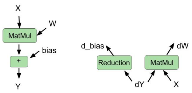
The cuBLAS library recently introduced a new type of fusion: fusing bias gradient computation and weight gradient computation in the same kernel.
In this round, we used this cuBLAS feature to fuse these two operations in the backward pass. We also fused bias addition and matrix multiplication in the forward pass. Figure 1 shows the fused operations for the forward pass and backward pass.
Improved fused multihead attention
In the previous round, we implemented fusing of the multihead attention module. This module used parallelism across the num_sequences and num_heads variables. This means that there are a total of num_sequences*num_heads thread blocks that are scheduled simultaneously on different streaming multiprocessors (SMs) on the GPU. num_heads is 16 in the MLPerf BERT model, and when num_sequences is smaller than 6, there are not enough thread blocks to fill the GPU, limiting the parallelism.
In this round, we improved these kernels by introducing slicing across the sequence dimension for batched matrix multiplications required for attention computation, which helped increase the parallelism proportionately. This optimization resulted in an ~8% end-to-end speedup for max-scale training scenarios, where the per-chip batch size is small.
Full iteration graph capture with CUDA Graphs
As mentioned in the previous section on CUDA Graphs, in this round, we captured the full iteration of BERT into a single CUDA graph. This was possible due to CUDA Graphs support in the NCCL communications library, as well as the PyTorch framework. This resulted in ~3% end-to-end savings due to reduced CPU latency and jitter at scale. On top of that, we also leveraged NCCL user-buffer preregistration feature when CUDA Graphs is used, resulting in another ~2% of end-to-end performance improvement.
Setting model parameter buffers to point to a contiguous flat buffer
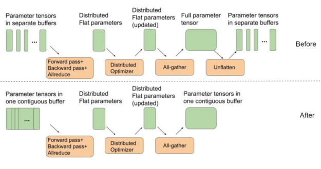
BERT uses a distributed optimizer to speed up optimization steps. For best all-gather performance, the intermediate buffers used in a distributed optimizer for weight parameters should all be part of a single contiguous flat buffer. This way, instead of running several all-gather functions on small separate tensors, we can better use GPU interconnects by running all-gather for one large message.
On the other hand, PyTorch by default allocates separate buffers for each of the model’s parameter tensors to be used during the forward pass. This requires an extra “unflattening” step, as shown in Figure 2, between the end of an iteration and the beginning of the next one.
In this MLPerf round, we used a single contiguous buffer where each parameter tensor is placed next to each other as part of one big buffer. This removes the need for the extra unflattening step, as shown in Figure 2. This optimization results in ~4% end-to-end performance savings for BERT at max-scale configurations, where the cost of optimizer and parameter copies is most pronounced.
DLRM
HugeCTR, a recommendation system dedicated training framework, part of NVIDIA Merlin, continues to power NVIDIA DLRM submission.
Hybrid embedding index precomputing
In the previous MLPerf round, we implemented hybrid embedding to reduce the communication between GPUs.
Even though the hybrid embedding implemented in HugeCTR significantly reduces the communication traffic, it requires indices to be calculated to determine where to read and distribute the embedding vectors stored on each GPU. The index calculation only relies on the input data, which is prefetched onto the GPU a few iterations ahead. Therefore, in HugeCTR, index precomputing is leveraged as an optimization to hide the cost of computing the indices under the communication kernels of the previous iteration.
Sharing the same spirit as index precomputing in training iterations, the hybrid embedding indices for evaluation can be computed and cached when the evaluation is performed for the first time. They can be reused for the remaining evaluations, which completely removes the cost of computing the indices for subsequent evaluations.
Better overlapping between communication and computation
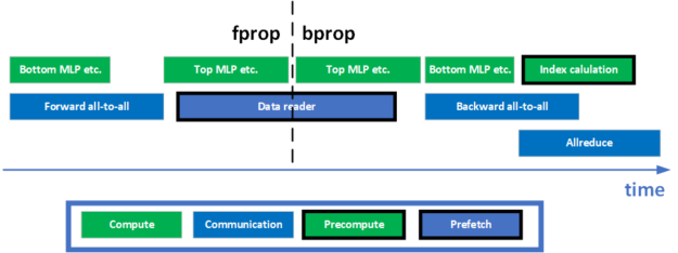
In DLRM, to facilitate model-parallel training, two all-to-all collectives are needed in the forward and backward phases, respectively. In addition, there is an all-reduce collective at the end of the training for the data-parallel part of the model. How to overlap computation with these communication collectives is key to achieve a high utilization of the GPU, and a high training throughput. A few optimizations have been made to enable a better overlap. Figure 3 shows a simplified timeline for one training iteration.
In the forward propagation phase, the bottom MLP is performed while the forward all-to-all kernel is waiting for the data to arrive. In the backward propagation phase, all-reduce and all-to-all are overlapped to increase the utilization of the network. The index precomputation is also scheduled to overlap with these two communication collectives to use the idle resources on the GPU, maximizing the training throughput.
Asynchronous weight gradients computing
The data gradient computation and weight gradient computation of an MLP are two independent branches of computations that share the same input. Unlike the data gradients, weight gradients are not needed until the gradient all-reduce. Thanks to the flexibility of the GPU in scheduling kernels, these two computations are performed in parallel in HugeCTR, maximizing the utilization of the GPU.
Better fusions
Kernel fusion is an effective way to reduce trips to memory, improving the GPU utilization. Many fusion patterns have been leveraged in DLRM to achieve better performance previously. For example, the data gradient calculation, ReLU backward operation and bias gradient calculation can be fused together in HugeCTR through cuBLAS. Such a cross-layer fusion pattern leaves the last bias gradient computation unfused.
In this round, the GEMM and bias gradient fusion supported in cuBLAS is leveraged to fuse the bias gradient computation into the weight gradient computation for the last layer of an MLP.
Another fusion example is weight conversion fusion. To support mixed-precision training, the FP32 master weights must be casted into FP16 weights during training. As an optimization, this precision casting is fused with the SGD optimizer in HugeCTR. Whenever an FP32 master weight is updated, it writes out an FP16 version of the updated weight into the memory, eliminating the need for a separate kernel for doing the conversion.
Mask R-CNN
NEEDS LEAD-IN SENTENCE
Using NHWC layout for all the convolutional layers
The ResNet-50 backbone has used the NHWC layout for a long time, but the rest of the model used NCHW up until now.
This round we were able to switch the FPN module (which immediately follows the ResNet-50 backbone) to NHWC. Running FPN in NHWC means we can transpose the outputs instead of the inputs, which is more efficient because the inputs are much larger than the outputs. This change boosted the performance by 4-5% for the max-scale configurations.
Using dedicated nodes exclusively for evaluation for multinode scenario
Although evaluation overlaps with training, Mask R-CNN evaluation is a resource-intensive process. Inevitably, training performance suffers slightly when evaluation is running simultaneously. For max-scale configurations, evaluation takes almost as long as training. Having evaluation constantly running in the background significantly affects the training performance.
One way to overcome this issue is to use a separate set of nodes for evaluation, that is, one set of nodes does training and a smaller set of nodes does evaluation. Implementing this change for max-scale configurations boosted the end-to-end performance by 12%.
Using multithreaded COCO evaluation
The COCO evaluation function consumes most of the evaluation time and is run separately on the bounding box and segmentation mask results. A couple of rounds ago we overlapped these two evaluation calls by running them in multiple processes.
This round, we enabled multi-threaded processing with openmp for the COCO evaluation loop. This is an optional feature in the NVIDIA version of the COCO API software. The evaluation loop can be parallelized by providing an optional argument that specifies the desired number of threads. This optimization improves evaluation speed by about 10%, but only the last evaluation is exposed, so the effect on end-to-end time is much smaller, about 0.5%.
Two-stage top-K computation with quadrupled occupancy for small batch-size runs
We make a couple of top-K calls in Mask R-CNN that take a long time due to low occupancy. The number of cooperative thread arrays, or CTAs (thread blocks) launched by the top-K kernel is proportional to the per-GPU batch size. Max-scale configurations use a per-GPU batch size of 1, which results in only five CTAs being launched. Each CTA is assigned one SM, while the A100 has more than 100 SMs, suggesting low utilization of the GPU.
To alleviate this, we implemented a two-stage approach:
- In the first stage, we split the input into four equal parts and then we do top-K on each part with a single call.
- In the second stage, we concatenate the four temporary results and take top-K of that.
This yields the same result as before but runs more than 3x faster because we are now launching 20 CTAs instead of 5 in the first stage. Dividing the input further makes the first stage faster, but also makes the second stage slower.
Splitting the input eight ways instead of four means that 40 CTAs are launched instead of 20 in the first stage. The first stage completes in half the time but, unfortunately, the second stage becomes so much slower that overall performance is better with a four-way split. Implementing a four-way split for the max-scale configuration resulted in a 3-4% performance boost.
Overlapping loss computations for mask head, bounding-box head, and RPN-head
Most of the GPU kernels launched by Mask R-CNN suffer from low occupancy when the batch size is small. One way to alleviate this is to overlap execution of as many kernels as possible to take advantage of the GPU resources that would otherwise go idle.
Some of the loss calculations can be done simultaneously. This is true for mask-head loss, bounding-box loss, and RPN-head loss, so we place each of these three loss calculations on different CUDA streams so that they can be executed simultaneously. This boosted the performance by about 5% for max-scale configurations.
3D-UNet
Vectorized concatenate and split operation
3D-UNet uses concatenate operations to concatenate the decoder and encoder activations. This results in device-to-device copies for activation tensors in the forward and backward passes. We optimized these copies by using vectorized loads and stores, doing a 4x wider read/write operation. This speeds up the concat and split operators by over 2.4x, giving an end-to-end speedup of 4.7% on single node configuration and 1.3% on max-scale configuration.
Efficient spatial-parallel convolutions
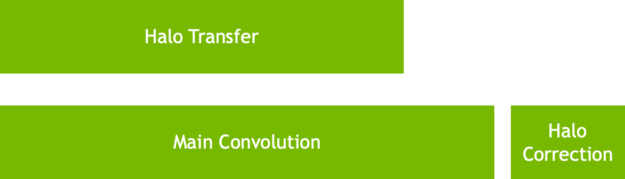
In MLPerf v1.0, we introduced spatial-parallel convolution, where we split the input activation across multiple GPUs (8 to be precise). The implementation of spatial-parallel convolution enabled us to hide the halo exchanges behind convolutions behind the convolution.
In MLPerf v1.1, we optimized the scheduling of communication and convolution operations so that we get a much better overlap between the launched communication and convolution kernels. While this makes sure that the halo exchanges are not exposed, it also helps reduce the jitter significantly. This optimized scheduling improved scores in max-scale configuration by over 25%.
Spatial-parallel loss calculations
3D-Unet uses the DICE loss and Softmax Cross Entropy loss as its loss functions. The DICE loss is defined as the following formula:
In this formula, 

In the max-scale configuration, because a single GPU works on just a slice of the image, each GPU holds only a slice of
Better configurations
We increased the global batch size to be a factor of dataset size. The DALI data loader library enables us to use the same shard to train for different epochs. This enables us to reduce the time it takes to cache the dataset in the GPU significantly.
Because each GPU loads much fewer images, the Bounding Box cache in DALI warms up much more quickly too. This optimization reduced the startup time significantly and resulted in 20% speedup over MLPerf v1.0.
Data-parallel async evaluation
As training gets faster, scaling evaluation to hide behind training becomes challenging. In MLPerf v1.1, the inferences on a single image were sharded across the GPUs to improve the evaluation scaling. The results of inferences were then all-gathered to form the final output. This enables the entire evaluation phase to be hidden behind training iterations.
Faster group instance norm
The multi-GPU Instancenorm kernel was improved significantly by parallelizing the inter-GPU communication of multiple channel-blocks and reducing the DRAM time of the kernel by vectorizing memory reads and writes. This resulted in throughput improvement of over 5% in the max-scale configuration.
ResNet-50
End-to-end CUDA graphs
For ResNet-50, as the benchmark scales out to >256 nodes, the per-GPU batch size reduces to a very small value, where the iteration time is only ~8-10ms. At these extremely small iteration times, it is critical to ensure there are no gaps in GPU execution arising from dependencies running on the CPU.
For MLPerfV1.1, we reduced jitter at scale by using end-to-end CUDA Graphs to capture an entire iteration across the forward pass, backward pass, optimizer, and Horovord/NCCL gradient all-reduce as a single graph. The use of CUDA Graphs provides a 6% performance benefit at max-scale training.
GBN
As the scale increases for ResNet50 and the local batch sizes decrease, to achieve the fastest possible convergence, we use the GBN technique. For every BatchNorm layer, the mean and variance is all-reduced among a group of GPUs.
For MLPerf v1.1, the performance of GBN within a single DGX node was significantly improved by parallelizing the inter GPU communication of multiple channel-blocks and reducing the DRAM time of the kernel by vectorizing memory reads and writes. This provided a 10% performance benefit at scale.
SSD
On-GPU image caching
Image networks make heavy use of image cropping and resizing to capture features that represent richer statistics of the dataset and to improve the generalization capability of the model.
In the previous MLPerf rounds, SSD used the NVIDIA Data Loading Library (DALI) image decoding features to decode only the cropped region of the JPG image. This feature avoids wasting time decoding the entire image, especially if the crop is small.
However, this means that this cropped image is only used one time as the image is not cached in memory. Future uses of the original image will likely have different cropped regions, meaning that the original image will be decoded each time it is used. This behavior leads to jitter across GPUs as the decoding cost varies greatly on the size of the region required by the crop. This is particularly pronounced for scale-out scenarios.
For this round, we took advantage of the 80-GB memory capacity available to each NVIDIA A100 80-GB GPU by using another DALI feature that decodes the entire image and caches it in memory. This enables future uses of the same image to avoid the decoding cost and instead pick the cropped region directly from memory. Doing this is cheaper than decoding the cropped region each time and has much less run-to-run and device-to-device variation in execution time.
Overall, this optimization resulted in 2% end-to-end performance improvement in our single node configuration and ~5% improvement in our efficient-scale configuration, which is in between single-node and max-scale in terms of scale.
GBN for SSD
SSD also took advantage of the GBN improvements implemented in ResNet-50, which gave a ~4% E2E improvement in our max-scale configuration.
RNN-T
More optimized apex transducer
The transducer module in apex has been further optimized to improve the training throughput. Two optimizations have been added to the transducer joint and transducer loss module, respectively.
Transducer joint, ReLU, and dropout are three consecutive memory-bound operations in RNN-T. As an optimization, ReLU and dropout have been fused with the transducer joint in the apex.contrib.transducer.TransducerJoint module in apex, effectively cutting the trips to the memory.
The backward propagation of the transducer loss is a memory-intensive operation. An optimization of vectorizing the loads and stores in the backward operation has been added to apex.contrib.transducer.TransducerLoss in apex, improving the memory bandwidth utilization of the kernel.
More data preprocessing on GPU
Preprocessing the next batch on the CPU while the GPU is busy with a forward and backward pass can hide data preprocessing time. This is ideal. However, when data preprocessing is compute-intensive, the preprocessing time on the CPU might get exposed.
DALI can help unload the CPU by computing parts of the preprocessing on GPU, leveraging the massively parallel processing nature of the GPU. In this submission, the silence trimming operation was moved to GPU, improving the training throughput.
Conclusion
Building upon the well-established and proven NVIDIA A100 GPU and NVIDIA DGX A100 platforms, optimization across the stacks continues to deliver performance improvements across the board for NVIDIA platform-based submissions in this round of MLPerf v1.1 training benchmark.
It is worth reiterating that the NVIDIA platform has been the only solution to make submissions across all workloads in the MLPerf benchmarking suite, demonstrating both industry-leading performance and versatility.
All software used for NVIDIA submissions is available from the MLPerf repository, to enable you to reproduce our benchmark results. We constantly add these cutting-edge MLPerf improvements into our deep learning frameworks containers available on NGC, our software hub for GPU-optimized applications.