Categories
Offsites

LaMDA: Towards Safe, Grounded, and High-Quality Dialog Models for Everything

Language models are becoming more capable than ever before and are helpful in a variety of tasks — translating one language into another, summarizing a long document into a brief highlight, or answering information-seeking questions. Among these, open-domain dialog, where a model needs to be able to converse about any topic, is probably one of the most difficult, with a wide range of potential applications and open challenges. In addition to producing responses that humans judge as sensible, interesting, and specific to the context, dialog models should adhere to Responsible AI practices, and avoid making factual statements that are not supported by external information sources.

Today we’re excited to share recent advances in our “LaMDA: Language Models for Dialog Applications” project. In this post, we’ll give an overview on how we’re making progress towards safe, grounded, and high-quality dialog applications. LaMDA is built by fine-tuning a family of Transformer-based neural language models specialized for dialog, with up to 137B model parameters, and teaching the models to leverage external knowledge sources.

Objectives & Metrics
Defining objectives and metrics is critical to guide training dialog models. LaMDA has three key objectives — Quality, Safety, and Groundedness — each of which we measure using carefully designed metrics:

Quality: We decompose Quality into three dimensions, Sensibleness, Specificity, and Interestingness (SSI), which are evaluated by human raters. Sensibleness refers to whether the model produces responses that make sense in the dialog context (e.g., no common sense mistakes, no absurd responses, and no contradictions with earlier responses). Specificity is measured by judging whether the system’s response is specific to the preceding dialog context, and not a generic response that could apply to most contexts (e.g., “ok” or “I don’t know”). Finally, Interestingness measures whether the model produces responses that are also insightful, unexpected or witty, and are therefore more likely to create better dialog.

Safety: We’re also making progress towards addressing important questions related to the development and deployment of Responsible AI. Our Safety metric is composed of an illustrative set of safety objectives that captures the behavior that the model should exhibit in a dialog. These objectives attempt to constrain the model’s output to avoid any unintended results that create risks of harm for the user, and to avoid reinforcing unfair bias. For example, these objectives train the model to avoid producing outputs that contain violent or gory content, promote slurs or hateful stereotypes towards groups of people, or contain profanity. Our research towards developing a practical Safety metric represents very early work, and there is still a great deal of progress for us to make in this area.

Groundedness: The current generation of language models often generate statements that seem plausible, but actually contradict facts established in known external sources. This motivates our study of groundedness in LaMDA. Groundedness is defined as the percentage of responses with claims about the external world that can be supported by authoritative external sources, as a share of all responses containing claims about the external world. A related metric, Informativeness, is defined as the percentage of responses with information about the external world that can be supported by known sources, as a share of all responses. Therefore, casual responses that do not carry any real world information (e.g., “That’s a great idea”), affect Informativeness but not Groundedness. While grounding LaMDA generated responses in known sources does not in itself guarantee factual accuracy, it allows users or external systems to judge the validity of a response based on the reliability of its source.

LaMDA Pre-Training
With the objectives and metrics defined, we describe LaMDA’s two-stage training: pre-training and fine-tuning. In the pre-training stage, we first created a dataset of 1.56T words — nearly 40 times more words than what were used to train previous dialog models — from public dialog data and other public web documents. After tokenizing the dataset into 2.81T SentencePiece tokens, we pre-train the model using GSPMD to predict every next token in a sentence, given the previous tokens. The pre-trained LaMDA model has also been widely used for natural language processing research across Google, including program synthesis, zero-shot learning, style transfer, as well as in the BIG-bench workshop.

LaMDA Fine-Tuning
In the fine-tuning stage, we train LaMDA to perform a mix of generative tasks to generate natural-language responses to given contexts, and classification tasks on whether a response is safe and high-quality, resulting in a single multi-task model that can do both. The LaMDA generator is trained to predict the next token on a dialog dataset restricted to back-and-forth dialog between two authors, while the LaMDA classifiers are trained to predict the Safety and Quality (SSI) ratings for the response in context using annotated data. During a dialog, the LaMDA generator first generates several candidate responses given the current multi-turn dialog context, and the LaMDA classifiers predict the SSI and Safety scores for every response candidate. Candidate responses with low Safety scores are first filtered out. Remaining candidates are re-ranked by their SSI scores, and the top result is selected as the response. We further filter the training data used for the generation task with LaMDA classifiers to increase the density of high-quality response candidates.

LaMDA generates and then scores a response candidate.
LaMDA handles arbitrary user input in a way that is sensible, specific, and interesting. Only LaMDA’s very first statement “Hello, I’m a friendly…” was hard coded to set the purpose of the dialog.

Factual Grounding
While people are capable of checking their facts by using tools and referencing established knowledge bases, many language models draw their knowledge on their internal model parameters only. To improve the groundedness of LaMDA’s original response, we collect a dataset of dialogs between people and LaMDA, which are annotated with information retrieval queries and the retrieved results where applicable. We then fine-tune LaMDA’s generator and classifier on this dataset to learn to call an external information retrieval system during its interaction with the user to improve the groundedness of its responses. While this is very early work, we’re seeing promising results.

Zero-shot domain adaptation: cherry-picked, but real example of LaMDA pretending to be Mount Everest, by simply setting its initial message to be “Hi I’m Mount Everest. What would you like me to know about me?” Everest LaMDA is shown providing educational and factually correct responses.

Evaluation
In order to quantify progress against our key metrics, we collect responses from the pre-trained model, fine-tuned model, and human raters (i.e., human-generated responses) to multi-turn two-author dialogs, and then ask a different set of human raters a series of questions to evaluate these responses against the Quality, Safety, and Groundedness metrics.

We observe that LaMDA significantly outperforms the pre-trained model in every dimension and across all model sizes. Quality metrics (Sensibleness, Specificity, and Interestingness, in the first column below) generally improve with the number of model parameters, with or without fine-tuning. Safety does not seem to benefit from model scaling alone, but it does improve with fine-tuning. Groundedness improves as model size increases, perhaps because larger models have a greater capacity to memorize uncommon knowledge, but fine-tuning allows the model to access external knowledge sources and effectively shift some of the load of remembering knowledge to an external knowledge source. With fine-tuning, the quality gap to human levels can be narrowed, though the model’s performance remains below human levels in safety and groundedness.

Comparing the pre-trained model (PT), fine-tuned model (LaMDA) and human-rater-generated dialogs (Human) across Sensibleness, Specificity, Interestingness, Safety, Groundedness, and Informativeness. The test sets used to measure Safety and Groundedness were designed to be especially difficult.

Future Research & Challenges
LaMDA’s level of Sensibleness, Specificity and Interestingness unlocks new avenues for understanding the benefits and risks of open-ended dialog agents. It also presents encouraging evidence that key challenges with neural language models, such as using a safety metric and improving groundedness, can improve with larger models and fine-tuning with more well-labeled data. However, this is very early work, and there are significant limitations. Exploring new ways to improve our Safety metric and LaMDA’s groundedness, aligned with our AI Principles, will continue to be our main areas of focus going forward.

Acknowledgements
We’d to like to thank everyone for contributing to the project and paper, including: Blaise Aguera-Arcas, Javier Alberca, Thushan Amarasiriwardena, Lora Aroyo, Martin Baeuml, Leslie Baker, Rachel Bernstein, Taylor Bos, Maarten Bosma, Jonas Bragagnolo, Alena Butryna, Bill Byrne, Chung-Ching Chang, Zhifeng Chen, Dehao Chen, Heng-Tze Cheng, Ed Chi, Aaron Cohen, Eli Collins, Marian Croak, Claire Cui, Andrew Dai, Dipanjan Das, Daniel De Freitas, Jeff Dean, Rajat Dewan, Mark Diaz, Tulsee Doshi, Yu Du, Toju Duke, Doug Eck, Joe Fenton, Noah Fiedel, Christian Frueh, Harish Ganapathy, Saravanan Ganesh, Amin Ghafouri, Zoubin Ghahramani, Kourosh Gharachorloo, Jamie Hall, Erin Hoffman-John, Sissie Hsiao, Yanping Huang, Ben Hutchinson, Daphne Ippolito, Alicia Jin, Thomas Jurdi, Ashwin Kakarla, Nand Kishore, Maxim Krikun, Karthik Krishnamoorthi, Igor Krivokon, Apoorv Kulshreshtha, Ray Kurzweil, Viktoriya Kuzmina, Vivek Kwatra, Matthew Lamm, Quoc Le, Max Lee, Katherine Lee, Hongrae Lee, Josh Lee, Dmitry Lepikhin, YaGuang Li, Yifeng Lu, David Luan, Daphne Luong, Laichee Man, Jianchang (JC) Mao, Yossi Matias, Kathleen Meier-Hellstern, Marcelo Menegali, Muqthar Mohammad,, Muqthar Mohammad, Alejandra Molina, Erica Moreira, Meredith Ringel Morris, Maysam Moussalem, Jiaqi Mu, Tyler Mullen, Tyler Mullen, Eric Ni, Kristen Olson, Alexander Passos, Fernando Pereira, Slav Petrov, Marc Pickett, Roberto Pieraccini, Christian Plagemann, Sahitya Potluri, Vinodkumar Prabhakaran, Andy Pratt, James Qin, Ravi Rajakumar, Adam Roberts, Will Rusch, Renelito Delos Santos, Noam Shazeer, RJ Skerry-Ryan, Grigori Somin, Johnny Soraker, Pranesh Srinivasan, Amarnag Subramanya, Mustafa Suleyman, Romal Thoppilan, Song Wang, Sheng Wang, Chris Wassman, Yuanzhong Xu, Yuanzhong Xu, Ni Yan, Ben Zevenbergen, Vincent Zhao, Huaixiu Steven Zheng, Denny Zhou, Hao Zhou, Yanqi Zhou, and more.

Categories
Misc

How to call predict() in eager mode (tf1 and tf2 compatibility issues)

I’m trying to perform an adversarial attack using [this demo] on my detection model created with tensorflow/keras. The problem is that the script I’m trying to use was written with TF1 in mind, whereas I’ve created my model with TF2.

When I feed my model into the script I’m seeing the following error:

ValueError: Calling `Model.predict` in graph mode is not supported when the `Model` instance was constructed with eager mode enabled. Please construct your `Model` instance in graph mode or call `Model.predict` with eager mode enabled.

I’ve already learned that this is because different TF versions used different modes by default. Could you give me a tip on what can I do to convert my model to the fitting mode?

submitted by /u/Piotrek1
[visit reddit] [comments]

Categories
Misc

Wrap up of Advent of Code 2021 in pure TensorFlow

Wrap up of Advent of Code 2021 in pure TensorFlow submitted by /u/pgaleone
[visit reddit] [comments]
Categories
Misc

Custom loss with images

Hi everyone, probably this is a silly question but I will appreciate if someone takes the time to answer it please.

I’m trying to build a custom loss function, and for now as a dummy I’m just trying to build a MSE function and compare it with the in-built MSE.

My code is just an autoencoder that receives 2D images with a batch size of 128, so when verify y_true I obtain a tensor like this: [128, 256, 256] where the 128 is batch size and the other two are the dimensions.

So, when I was looking for the MSE custom loss and compared it with the in-built one, I realised that they’re doing something like this:

diff = math_ops.squared_difference(y_pred, y_true) loss = K.mean(diff, axis=-1) loss = loss/10 

Then I get a vector as a loss function as this: [128,256], so my question is: is this right? shouldn’t loss be an scalar value instead of a vector?, should I use the whole 3D tensor instead of only 2 components in the 2nd line?

I’m kinda lost and since I don’t understand this I cannot move forward on my project.

submitted by /u/DaSpaceman245
[visit reddit] [comments]

Categories
Misc

Training Custom TFDS Dataset

Hi, I am working on a classification task for audio data with a custom dataset. i am trying to use the leaf audio github on my own dataset, which runs on the speech commands tfds dataset. i created my own tfds dataset for my custom data, following the exact same setup as the speech commands data. however, i am running into an issue as the dataset is stored in the PrefetchDataset format, and I do not know how to access the data for model.fit . i have researched ways to fix this error and the solutions have not worked, so i was wondering if anyone would be able to help me

submitted by /u/Kunnanada
[visit reddit] [comments]

Categories
Misc

Data Science Best Practices for an Intelligent Edge Solution

Learn industry insights and best practice for implementing data science with AI at the edge.Learn industry insights and best practice when implementing data science and AI at the edge. Learn industry insights and best practice for implementing data science with AI at the edge.
Whether your organization is new to data science or has a mature strategy in place, many come to a similar realization: Most data does not originate at the core. 

Scientists often want access to amounts of data that are unreasonable to securely stream to the data center in real time. Whether the distance is 10 miles or thousands of miles, the bounds of traditional IT infrastructure are simply not designed to stretch outside of fixed campuses. 

This has led organizations to realize that no data science strategy is complete without an edge strategy. 

Read on to learn industry insights on the benefits of coupling data science and edge computing, the challenges faced, solutions to these challenges, and register to view a demo of an edge architecture blueprint.

Edge Architectures 

Edge computing is a style of IT architecture that is typically employed to create systems that are tolerant of geographically distributed data sources and high latency and low-bandwidth interconnects. 

Due to restrictions imposed by the operating environment, computing systems designed in this way are typically identifiable by compromises on computational speed and high availability. 

Today, there are three types of edge architectures that are commonly being used by organizations: streaming data, edge preprocessing, and autonomous systems. 

Edge Architecture 1: Streaming data 

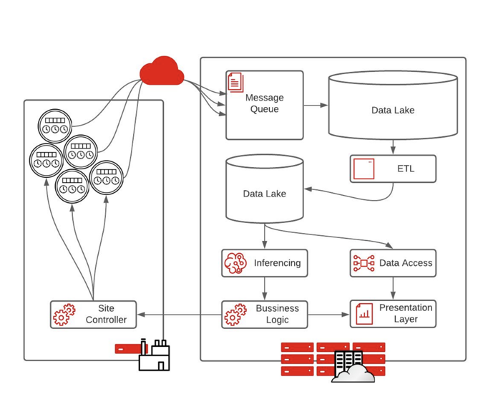
In a
Image 1: The streaming data architecture collects data at the edge and processes it in the cloud. 

Today, streaming data, the “classical big data” architecture, is the most popular prototypical architecture for organizations that are just starting to implement an edge strategy. This architecture starts with IoT devices, usually sensors, placed anywhere from a factory floor, hospital, or retail store. The data is then sent through the cloud to an IT system. 

As data processing abilities increase, the classic big data architecture can be a hindrance because of the level of infrastructure required and the large quantity of data that needs to move from the edge to core.

Edge Architecture 2: Edge Pre-Processing 

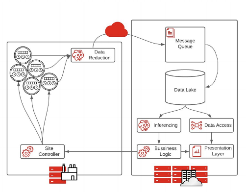
This image shows what an
Image 2: Edge-preprocessing models are considered to be a hybrid edge and cloud model. 

The edge preprocessing model is the most common architecture for organizations transitioning to the edge.

Instead of sensor data feeding directly into a pipeline running in the data center, data is fed into an intelligent data reduction application. This is usually an intelligent machine-learning algorithm that decides what data is important and needs to be sent back to the data center. 

Extraction, transformation, and loading (ETL) processes are less important in these architectures because data reduction has already occurred at the edge. Therefore, there is no need for two data lakes, and inference can happen more quickly. The result is faster execution on business logic. 

This is a good stepping stone for creating fully autonomous systems, allowing for an unlimited amount of data compression.

Edge Architecture 3: Autonomous Systems 

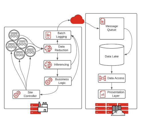
The image shows an
Image 3: Autonomous systems process data at the edge and are characterized by rapid decision-making.  

Fully autonomous systems are characterized by sensors collecting data at the edge to make rapid decisions with low latency. With no time to send data back to a data center or cloud to make a proper decision, processing happens at the edge and actions are taken automatically. 

With this architecture, every step of the pipeline is sent to a logging mechanism to record the decisions made at the edge. The batch logging will send messages to the cloud or core data center to allow for analytics and system adjustments on the decisions made. 

Industry Insights for Building the Intelligent Edge 

Building an intelligent edge solution is not just about pushing a container to tens or thousands of sites. While it may seem like a trivial task, your organization’s success relies heavily on the infrastructure that you put in place, not just the data science.  

There are many complexities that need to be taken into consideration when building an intelligent edge solution such as scale, interoperability, and consistency. 

Suggested technologies to build intelligent solutions are: 

  • Linux edge systems 
  • Containers 
  • Kubernetes 
  • Messaging protocols (Kafka, MQTT, BYO) 

Edge Infrastructure in Practice 

As organizations look to meet their business needs and enable data science to drive innovation, your options should not be limited to your architecture. Implementing an edge architecture will help you future-proof your platform against new use cases and technologies. 

While it is helpful to understand where your architecture stands among different stages of edge implementation, it is often best to view a live demonstration.  

For more information, view our webinar, “Data Scientists on the Loose: Lessons Learned while Enabling the Intelligent Edge” for best practice regarding how to implement a Kubernetes system at the edge and the capabilities it can give your organization.   

Or, learn more about edge computing and data science

Categories
Misc

Scientists Develop 3D Simulation of a Living Cell

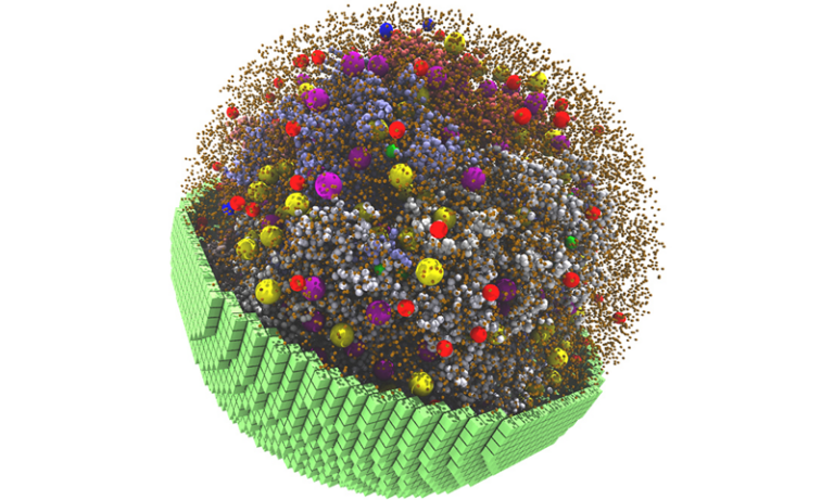
Researchers from the University of Illinois at Urbana-Champaign developed GPU-accelerated software to simulate a 2-billion-atom cell that metabolizes and grows like a living cell.

Categories
Misc

Natural Language Processing First Steps: How Algorithms Understand Text

This post shows how NLP in Text is converted into vectors to be compatible with ML and other algorithms.

This article will discuss how to prepare text through vectorization, hashing, tokenization, and other techniques, to be compatible with machine learning (ML) and other numerical algorithms. I’ll explain and demonstrate the process.

Natural Language Processing (NLP) applies Machine Learning (ML) and other techniques to language. However, machine learning and other techniques typically work on the numerical arrays called vectors representing each instance (sometimes called an observation, entity, instance, or row) in the data set.  We call the collection of all these arrays a matrix; each row in the matrix represents an instance. Looking at the matrix by its columns, each column represents a feature (or attribute).

So far, this language may seem rather abstract if one isn’t used to mathematical language. However, when dealing with tabular data, data professionals have already been exposed to this type of data structure with spreadsheet programs and relational databases. 

After all, spreadsheets are matrices when one considers rows as instances and columns as features. For example, consider a dataset containing past and present employees, where each row (or instance) has columns (or features) representing that employee’s age, tenure, salary, seniority level, and so on.

Terminology

The first problem one has to solve for NLP is to convert our collection of text instances into a matrix form where each row is a numerical representation of a text instance — a vector. But, in order to get started with NLP, there are several terms that are useful to know. Let’s introduce them.

In NLP, a single instance is called a document, while a corpus refers to a collection of instances. Depending on the problem at hand, a document may be as simple as a short phrase or name or as complex as an entire book.

One has to make a choice about how to decompose our documents into smaller parts, a process referred to as tokenizing our document. It follows that this process produces tokens. Tokens are the units of meaning the algorithm can consider. The set of all tokens seen in the entire corpus is called the vocabulary.

A common choice of tokens is to simply take words; in this case, a document is represented as a bag of words (BoW). More precisely, the BoW model scans the entire corpus for the vocabulary at a word level, meaning that the vocabulary is the set of all the words seen in the corpus. Then, for each document, the algorithm counts the number of occurrences of each word in the corpus.

Most words in the corpus will not appear for most documents, so there will be many zero counts for many tokens in a particular document. Conceptually, that’s essentially it, but an important practical consideration to ensure that the columns align in the same way for each row when we form the vectors from these counts. In other words, for any two rows, it’s essential that given any index k, the kth elements of each row represent the same word.

An example

Before getting into the details of how to assure that rows align, let’s have a quick look at an example done by hand. We’ll see that for a short example it’s fairly easy to ensure this alignment as a human. Still, eventually, we’ll have to consider the hashing part of the algorithm to be thorough enough to implement — I’ll cover this after going over the more intuitive part.

Suppose our corpus is the following four sentences1:

   “This is the first document.”

    “This document is the second document.”

    “And this is the third one.”

    “Is this the first document?

Preprocessing

Let’s apply some preprocessing to remove case and punctuation:

“this is the first document”

    “this document is the second document”

    “and this is the third one”

    “is this the first document”

Tokenization

Let’s tokenize the preprocessed documents by designating each word as a token:

“this”, “is”, “the”, “first”, “document”

    “this”, “document”, “is”, “the”, “second”, “document”

    “and”, “this”, “is”, “the”, “third”, “one”

    “is”, “this”, “the”, “first”, “document”

Getting the vocabulary

Scanning through the corpus and getting each unique word, we can form our vocabulary:

“this”, “is”, “the”, “first”, “document”, “second”, “and”, “third”, “one”

Vectorization

Let’s count the number of occurrences of each word in each document.

“this”: 1, “is”: 1, “the”: 1, “first”: 1, “document”: 1, “second”: 0, “and”: 0, “third”: 0, “one”: 0

“this”:1, “is”: 1, “the”: 1, “first”: 0, “document”: 2, “second”: 1, “and”: 0, “third”: 0, “one”: 0

“this”: 1, “is”: 1, “the”: 1, “first”: 0, “document”: 0, “second”: 0, “and”: 1, “third”: 1, “one”: 1

“this”: 1, “is”: 1, “the”: 1, “first”: 1, “document”: 1, “second”: 0, “and”: 0, “third”: 0, “one”: 0

Let’s collect this into a table.

This is the first document second and third one
1 1 1 1 1 0 0 0 0
1 1 1 0 2 1 0 0 0
1 1 1 0 0 0 1 1 1
1 1 1 1 1 0 0 0 0

If we ignore the header, this is the matrix we were looking for.

Hashing

It is worth noting that permuting the row of this matrix and any other design matrix (a matrix representing instances as rows and features as columns) does not change its meaning. The same is true for column permutations. Depending on how we map a token to a column index, we’ll get a different ordering of the columns, but no meaningful change in the representation.

This process of mapping tokens to indexes such that no two tokens map to the same index is called hashing2. A specific implementation is called a hash, hashing function, or hash function.

Vocabulary based hashing

While doing vectorization by hand, we implicitly created a hash function. Assuming a 0-indexing system, we assigned our first index, 0, to the first word we had not seen. Then we incremented the index and repeated the process. Our hash function mapped “this” to the 0-indexed column, “is” to the 1-indexed column and “the” to the 3-indexed columns. A vocabulary-based hash function has certain advantages and disadvantages.

Advantages of vocabulary based hashing

Using the vocabulary as a hash function allows us to invert the hash. This means that given the index of a feature (or column), we can determine the corresponding token. One useful consequence is that once we have trained a model, we can see how certain tokens (words, phrases, characters, prefixes, suffixes, or other word parts) contribute to the model and its predictions. We can therefore interpret, explain, troubleshoot, or fine-tune our model by looking at how it uses tokens to make predictions. We can also inspect important tokens to discern whether their inclusion introduces inappropriate bias to the model.

Let’s consider the artifacts produced by some machine learning models. For example, if we use a Logistic Regression model, we can interpret the coefficient associated with each feature as its effects on the model’s prediction. Random forest models yield feature importances, which tell us how often decision trees in the random forest use each feature to make decisions. Likewise, a Naive Bayes model produces the probability that a feature is non-zero for a specified class.

The power of vocabulary-based vectorization lies in understanding which token each feature represents. So, instead, with a Logistic Regression model, we can see how strongly each token affects the prediction. With Random forests, we get feature importance associated with each token, which tells us how often the decision trees in the random forest make decisions using each token. With naive Bayes, we can extract the probability of a certain token appearing in documents of each class.

If we see that seemingly irrelevant or inappropriately biased tokens are suspiciously influential in the prediction, we can remove them from our vocabulary. If we observe that certain tokens have a negligible effect on our prediction, we can remove them from our vocabulary to get a smaller, more efficient and more concise model.

Disadvantages of vocabulary based hashing

There are a few disadvantages with vocabulary-based hashing, the relatively large amount of memory used both in training and prediction and the bottlenecks it causes in distributed training.

One downside to vocabulary-based hashing is that the algorithm must store the vocabulary. With large corpuses, more documents usually result in more words, which results in more tokens. Longer documents can cause an increase in the size of the vocabulary as well.

On a single thread, it’s possible to write the algorithm to create the vocabulary and hashes the tokens in a single pass. However, effectively parallelizing the algorithm that makes one pass is impractical as each thread has to wait for every other thread to check if a word has been added to the vocabulary (which is stored in common memory). Without storing the vocabulary in common memory, each thread’s vocabulary would result in a different hashing and there would be no way to collect them into a single correctly aligned matrix.

A better way to parallelize the vectorization algorithm is to form the vocabulary in a first pass, then put the vocabulary in common memory and finally, hash in parallel. This approach, however, doesn’t take full advantage of the benefits of parallelization. Additionally, as mentioned earlier, the vocabulary can become large very quickly, especially for large corpuses containing large documents.

Mathematical hashing

Fortunately, there is an alternative way of hashing tokens: hash each instance with a non-cryptographic mathematical hash function. This type of hash function uses a combination of arithmetic, modular arithmetic, and algebra to map objects (represented by their bits) to a known range of integers or(bits). Since the range is known, the maximum value determines how many columns are in the matrix. Generally, the range is quite large, but for most rows, most columns will be 0. Therefore, with a sparse representation, the memory required to store the matrix will be minimal, and algorithms can efficiently handle sparse matrix-based operations.

Further, since there is no vocabulary, vectorization with a mathematical hash function doesn’t require any storage overhead for the vocabulary. The absence of a vocabulary means there are no constraints to parallelization and the corpus can therefore be divided between any number of processes, permitting each part to be independently vectorized. Once each process finishes vectorizing its share of the corpuses, the resulting matrices can be stacked to form the final matrix. This parallelization, which is enabled by the use of a mathematical hash function, can dramatically speed up the training pipeline by removing bottlenecks.

Although the use of mathematical hash functions can reduce the time taken to produce feature vectors, it does come at a cost, namely the loss of interpretability and explainability. Because it is impossible to map back from a feature’s index to the corresponding tokens efficiently when using a hash function, we can’t determine which token corresponds to which feature. So we lose this information and therefore interpretability and explainability.

Conclusion

In this article, we’ve seen the basic algorithm that computers use to convert text into vectors. We’ve resolved the mystery of how algorithms that require numerical inputs can be made to work with textual inputs.

Textual data sets are often very large, so we need to be conscious of speed. Therefore, we’ve considered some improvements that allow us to perform vectorization in parallel. We also considered some tradeoffs between interpretability, speed and memory usage.

By applying machine learning to these vectors, we open up the field of NLP (Natural Language Processing). In addition, vectorization also allows us to apply similarity metrics to text, enabling full-text search and improved fuzzy matching applications.


1This example comes from the SciKit-learn documentation: sklearn.feature_extraction.text.CountVectorizer

2In general, a hash function can map two entities to the same index. This is called a collision and should be an extremely rare occurrence for a hash function. Collisions are undesirable.

Categories
Misc

2021 Marked the Year of Virtual Worlds with Innovative Tools from NVIDIA Omniverse

An illustration with several Omniverse graphics highlights.NVIDIA Omniverse for virtual world building brought design collaboration and digital twins to center stage in 2021.An illustration with several Omniverse graphics highlights.

2021 was a landmark year for NVIDIA Omniverse, the multi-GPU enabled open platform for 3D design collaboration and real-time simulation. The platform became generally available to millions of creators, developers, and enterprise leaders looking to enhance 3D workflows and develop physically accurate digital twins. 

Recognized by TIME Magazine as a Best Invention, NVIDIA Omniverse is laying the foundation for robust virtual world creation and opening new paths to market for developers around the world.

Figure 1. The Omniverse Showroom app gives beginners a look into the foundational technologies of Omniverse, with new content regularly released.

With the growth of the platform last year came major new updates and releases for NVIDIA Omniverse Apps including Omniverse Create, Omniverse View, Omniverse Audio2Face, Omniverse Machinima, Omniverse Kaolin, and Omniverse XR Remote.

Powerful new features and frameworks include:

  • Omniverse Farm, a systems layer for users to orchestrate multiple computing resources to execute batch and interactive tasks. 
  • Omniverse VR, a new functionality coming to Omniverse Kit, with the world’s first full-fidelity, real-time ray traced VR
  • Omniverse Avatar, a developer’s technology platform for generating interactive virtual robots easily customizable for virtually any industry.
  • Omniverse Replicator, a powerful synthetic-data-generation engine that produces physically simulated synthetic data for training deep neural networks.
  • Connectors to applications like Autodesk 3ds Max, Autodesk Maya, and Epic Games’ Unreal Engine. Many more are in the pipeline, with an Adobe Substance 3D Material Extension coming soon. 
  • A custom Blender 3.0 Alpha release with advanced USD and MDL support, opening Omniverse to millions of Blender artists
  • Omniverse-ready USD assets from leading 3D marketplaces including TurboSquid by Shutterstock, CGTrader, Sketchfab, and Twinbru. 

Over 100,000 individual creators, designers, engineers, and students downloaded the NVIDIA Omniverse platform in 2021, while numerous leading companies explored NVIDIA Omniverse Enterprise to unite their teams, tools, and assets in a shared virtual space.  

Figure 2. NVIDIA Omniverse Enterprise is an end-to-end real-time collaboration and true-to-reality simulation platform for complex design workflows.

Some of the incredible work from the community, partners, customers, and senior NVIDIA Omniverse designers and engineers made in Omniverse are listed below.

Enterprise Highlights

Factory of the Future, BMW Group

At GTC in Spring of 2021, BMW Group debuted how they are using NVIDIA Omniverse Enterprise to create a digital twin of their automotive factory to reduce planning times and improve flexibility and precision.

Figure 3. Inside the factory simulation digital twin of BMW’s assembly system—powered by Omniverse.

Creator Highlights

A Graphics Flashback, Yenifer Macias

One of the #CreateYourRetroverse contest winners, Yenifer, used Omniverse Create, Adobe Substance Painter, Autodesk Maya, and ZBrush to design this nostalgic scene.

A retro-inspired arcade bedroom scene created with Omniverse.
Figure 4. A retro-inspired scene from the #CreateYourRetroverse by third-place winner Yenifer Macias.

Animated Films with Omniverse Audio2Face, Jae Solina

The creator behind the popular YouTube channel, JSFILMZ, Jae Solina is using NVIDIA Omniverse Audio2Face to save time and money on virtual production. “With Omniverse, I don’t have to wait a full week to render a 30-second animation,” Solina said. “The rendering speed in Omniverse is superb and saves me a lot of time, which is important when balancing my filmmaking, noncreative work, and family.”

Figure 5. Solina’s Omniverse Audio2Face Metahuman tutorial.

Character Creation, Benny Dee

Cartoon Network animator Benny Sokomba Dazhi, Benny Dee, uses the Reallusion iClone Omniverse Connector to streamline his 3D workflow. “The main challenges I faced when trying to meet deadlines were long render times and difficulties with software compatibility, but using an Omniverse Connector for Reallusion’s iClone app has been game-changing for my workflow,” he said.

Figure 6. Dazhi’s holiday video showcasing an Omniverse and Reallusion iClone workflow.

Developer Highlights

Connecting in the Metaverse: The Making of the GTC Keynote

At SIGGRAPH, NVIDIA premiered a documentary highlighting the creative minds and revolutionary technologies behind the GTC 2021 keynote, detailing how Omniverse was used to create a virtual version of NVIDIA’s CEO Jensen Huang.

Figure 7. See how a small team of artists were able to blur the lines between real and rendered with the NVIDIA GTC keynote in this behind-the-scenes documentary.

New Trainings and Tools for Developers Building on the Omniverse Platform

NVIDIA launched a new self-paced Deep Learning Institute training course, Getting Started with Universal Scene Description for Collaborative 3D Workflows, that familiarizes users with Universal Scene Description. The inaugural NVIDIA Omniverse Developer Day was also introduced at GTC in November, providing developers access to technical and business-focused sessions for building, extending, and connecting tools and platforms to the growing Omniverse ecosystem.

Resources

To learn more about NVIDIA Omniverse highlights from 2021, and to get an insider’s look at the 2022 product roadmap:

Categories
Misc

NVIDIA GPUs Enable Simulation of a Living Cell

Every living cell contains its own bustling microcosm, with thousands of components responsible for energy production, protein building, gene transcription and more. Scientists at the University of Illinois at Urbana-Champaign have built a 3D simulation that replicates these physical and chemical characteristics at a particle scale — creating a fully dynamic model that mimics the Read article >

The post NVIDIA GPUs Enable Simulation of a Living Cell appeared first on The Official NVIDIA Blog.