Warp is a Python API framework for writing GPU graphics and simulation code, especially within Omniverse.
Typically, real-time physics simulation code is written in low-level CUDA C++ for maximum performance. In this post, we introduce NVIDIA Warp, a new Python framework that makes it easy to write differentiable graphics and simulation GPU code in Python. Warp provides the building blocks needed to write high-performance simulation code, but with the productivity of working in an interpreted language like Python.
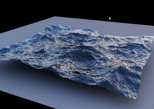
By the end of this post, you learn how to use Warp to author CUDA kernels in your Python environment and make use of some of the built-in high-level functionality that makes it easy to write complex physics simulations, such as an ocean simulation (Figure 1).
Figure 1. Ocean simulation in Omniverse using Warp
Installation
Warp is available as an open-source library from GitHub. When the repository has been cloned, you can install it using your local package manager. For pip, use the following command:
pip install warp
Initialization
After importing, you must explicitly initialize Warp:
import warp as wp
wp.init()
Launching kernels
Warp uses the concept of Python decorators to mark functions that can be executed on the GPU. For example, you could write a simple semi-implicit particle integration scheme as follows:
Because Warp is strongly typed, you should provide type hints to kernel arguments. To launch a kernel, use the following syntax:
    wp.launch(kernel=simple_kernel, # kernel to launch
              dim=1024,             # number of threads
              inputs=[a, b, c],     # parameters
              device="cuda")        # execution device
Unlike tensor-based frameworks such as NumPy, Warp uses a kernel-based programming model. Kernel-based programming more closely matches the underlying GPU execution model. It is often a more natural way to express simulation code that requires fine-grained conditional logic and memory operations. However, Warp exposes this thread-centric model of programming in an easy-to-use way that does not require low-level knowledge of GPU architecture.
Compilation model
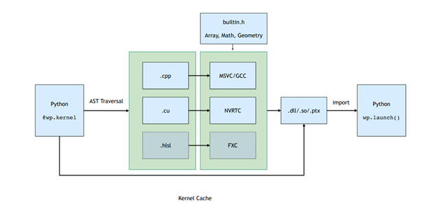
Launching a kernel triggers a just-in-time (JIT) compilation pipeline that automatically generates C++/CUDA kernel code from Python function definitions.
All kernels belonging to a Python module are runtime compiled into dynamic libraries and PTX. Figure 2. shows the compilation pipeline, which involves traversing the function AST and converting this to straight-line CUDA code that is then compiled and loaded back into the Python process.
Figure 2. Compilation pipeline for Warp kernels
The result of this JIT compilation is cached. If the input kernel source is unchanged, then the precompiled binaries are loaded in a low-overhead fashion.
Memory model
Memory allocations in Warp are exposed through the warp.array type. Arrays wrap an underlying memory allocation that may live in either host (CPU), or device (GPU) memory. Unlike tensor frameworks, arrays in Warp are strongly typed and store a linear sequence of built-in structures (vec3, matrix33, quat, and so on).
You can construct arrays from Python lists or NumPy arrays, or initialized, using a similar syntax to NumPy and PyTorch:
# allocate an uninitizalized array of vec3s
    v = wp.empty(length=n, dtype=wp.vec3, device="cuda")

    # allocate a zero-initialized array of quaternions
    q = wp.zeros(length=n, dtype=wp.quat, device="cuda")

    # allocate and initialize an array from a numpy array
    # will be automatically transferred to the specified device
    v = wp.from_numpy(array, dtype=wp.vec3, device="cuda")
Warp supports the __array_interface__, and __cuda_array_interface__ protocols, which allow zero-copy data views between tensor-based frameworks. For example, to convert data to NumPy use the following command:
# automatically bring data from device back to host
    view = device_array.numpy()
Features
Warp includes several higher-level data structures that make implementing simulation and geometry processing algorithms easier.
Meshes
Triangle meshes are ubiquitous in simulation and computer graphics. Warp provides a built-in type for managing mesh data that provide support for geometric queries, such as closest point, ray-cast, and overlap checks.
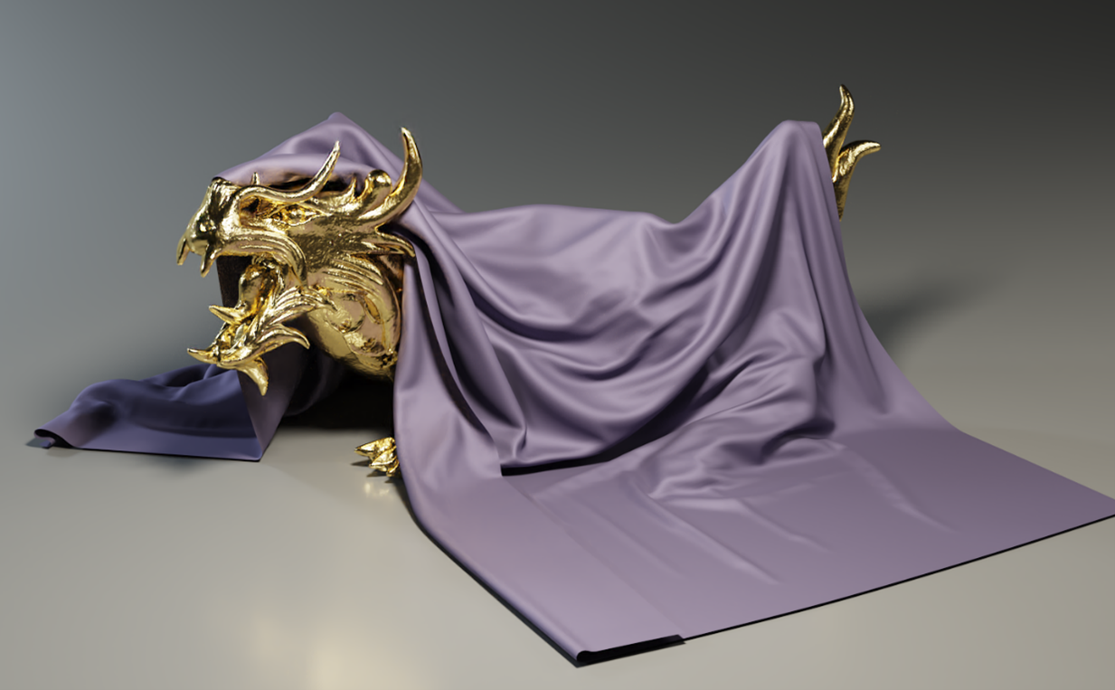
The following example shows how to use Warp to compute the closest point on a mesh to an array of input positions. This type of computation is the building block for many algorithms in collision detection (Figure 3). Warp’s mesh queries make it simple to implement such methods.
Figure 3. An example of collision detection against a complex object that uses closest-point mesh queries to test for contact between particles and the underlying object
Sparse volumes are incredibly useful for representing grid data over large domains, such as signed distance fields (SDFs) for complex objects or velocities for large-scale fluid flow. Warp includes support for sparse volumes defined using the NanoVDB standard. Construct volumes using standard OpenVDB tools such as Blender, Houdini, or Maya, and then sample inside Warp kernels.
You can create volumes directly from binary grid files on disk or in-memory, and then sample them using the volumes API:
wp.volume_sample_world(vol, xyz, mode)  # world space sample using interpolation mode
wp.volume_sample_local(vol, uvw, mode)  # volume space sample using interpolation mode
wp.volume_lookup(vol, ijk)              # direct voxel lookup
wp.volume_transform(vol, xyz)           # map point from voxel space to world space
wp.volume_transform_inv(vol, xyz)       # map point from world space to volume space
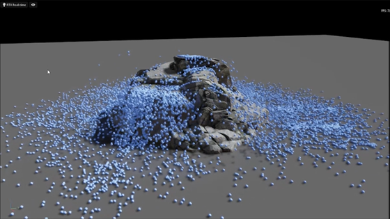
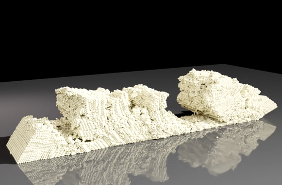
Figure 4. A particle simulation where the rock formation is represented as a sparse NanoVDB level set
Using volume queries, you can efficiently collide against complex objects with minimal memory overhead.
Hash grids
Many particle-based simulation methods, such as the discrete element method (DEM) or smoothed particle hydrodynamics (SPH), involve iterating over spatial neighbors to compute force interactions. Hash grids are a well-established data structure to accelerate these nearest neighbor queries and are particularly well suited to the GPU.
Hash grids are constructed from point sets as follows:
When hash grids are created, you can query them directly from within user kernel code as shown in the following example, which computes the sum of all neighbor particle positions:
@wp.kernel
def sum(grid : wp.uint64,
points: wp.array(dtype=wp.vec3),
output: wp.array(dtype=wp.vec3),
radius: float):
tid = wp.tid()
# query point
p = points[tid]
# create grid query around point
query = wp.hash_grid_query(grid, p, radius)
index = int(0)
sum = wp.vec3()
while(wp.hash_grid_query_next(query, index)):
neighbor = points[index]
# compute distance to neighbor point
dist = wp.length(p-neighbor)
if (dist
Figure 5 shows an example of a DEM granular material simulation for a cohesive material. Using the built-in hash-grid data structure allows you to write such a simulation in fewer than 200 lines of Python and runs at interactive rates for more than 100K particles.
Figure 5. An example of a DEM granular material simulation
Using the Warp hash-grid data allows you to easily evaluate the pairwise force interactions between neighboring particles.
Differentiability
Tensor-based frameworks, such as PyTorch and JAX, provide gradients of tensor computations and are well-suited for applications like ML training.
A unique feature of Warp is the ability to generate forward and backward versions of kernel code. This makes it easy to write differentiable simulations that can propagate gradients as part of a larger training pipeline. A common scenario is to use traditional ML frameworks for network layers, and Warp to implement simulation layers allowing for end-to-end differentiability.
When gradients are required, you should create arrays with requires_grad=True. For example, the warp.Tape class can record kernel launches and replay them to compute the gradient of a scalar loss function with respect to the kernel inputs:
After the backward pass has completed, the gradients with respect to the inputs are available through a mapping in the Tape object:
# gradient of loss with respect to input a
print(tape.gradients[a])
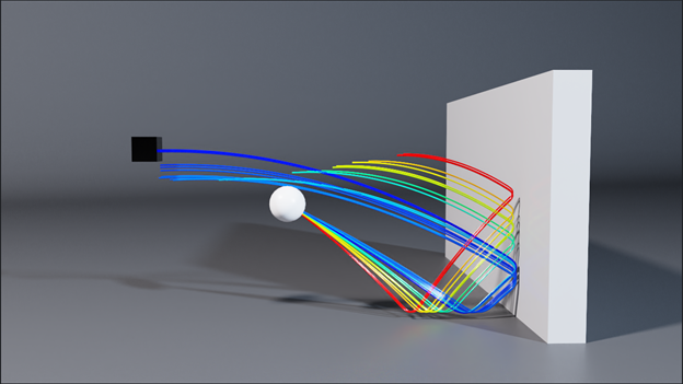
Figure 6. A trajectory optimization example where the initial velocity of the ball is optimized to hit the black target. Each line shows the result of one iteration of an LBFGS optimization step.
Summary
In this post, we presented NVIDIA Warp, a Python framework that makes it easy to write differentiable simulation code for the GPU. We encourage you to download the Warp preview release, share results, and give us feedback.
For more information, see the following resources:

 Warp is a Python API framework for writing GPU graphics and simulation code, especially within Omniverse.