
 Learn how using the combination of model parallel and data parallel
enables practitioners to train large-scale recommender systems in minutes instead of days.
Deep learning recommender systems often use large embedding tables. It can be difficult to fit them in GPU memory.
This post shows you how to use a combination of model parallel and data parallel training paradigms to solve this memory issue to train large deep learning recommender systems more quickly. I share the steps that my team took to efficiently train a 113 billion-parameter recommender system in TensorFlow 2, with the total size of all embeddings for this model being 421 GiB.
By splitting the model and embeddings between GPU and CPU, my team achieved a 43x speedup. However, distributing the embeddings across multiple GPUs resulted in an incredible 672x speedup. The significant speedup achieved by this multi-GPU method enables you to train large-scale recommender systems in minutes instead of days.
You may reproduce these results yourself using code available in the NVIDIA Deep Learning Examples GitHub Repository.
Model parallel training for embedding layers
In data-parallel training, each GPU stores the same copy of the model but trains on different data. This is convenient for many deep learning applications because of the easy implementation and relatively low communication overheads. However, this paradigm requires the weights of the neural network to fit onto a single device.
If the model size is larger than device memory, one approach is to split the model into subparts and train each subpart on a different GPU. This is called model-parallel training.
Each row of the table corresponds to a value of the input variable to map to a dense representation. Each column of the table represents a different dimension of the output space, representing a slice of one value through all the vectors. Because a typical deep learning recommender ingests multiple categorical features, it needs multiple embedding tables.
There are three approaches to implementing model parallelism for a recommender with multiple large embeddings:
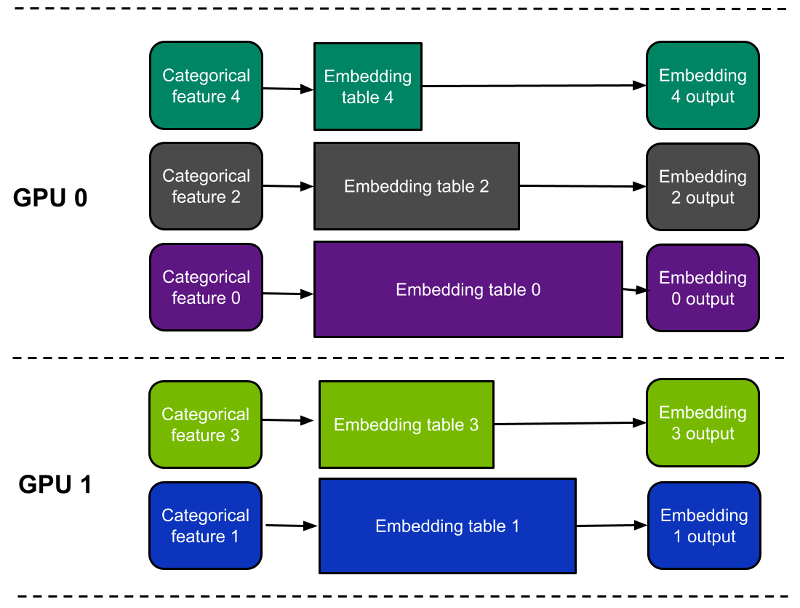
- Table-wise split–Each embedding table is placed entirely on a single device; each device holds only a subset of all embeddings. (Figure 1)
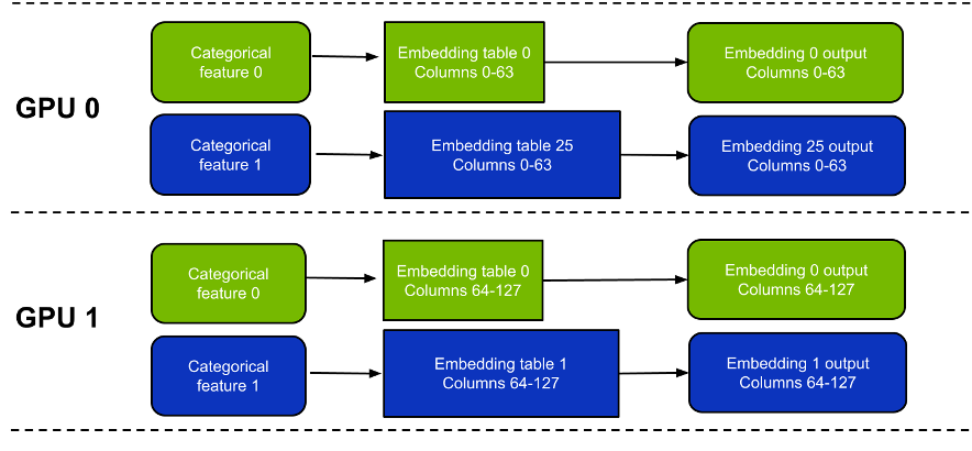
- Column-wise split–Each GPU holds a subset of columns from every embedding table. (Figure 2)
- Row-wise split–Each GPU holds a subset of rows from every embedding table.
Row-wise split is significantly more difficult to implement than the other two options because of load-balancing issues. In this post, I focus on table-wise split and column-wise split. Mixing and matching multiple approaches is a viable option but for simplicity, I do not focus on this throughout the post.
There are a few key differences between these approaches (Table 1). In short, table-wise split mode is slightly easier to use and potentially faster depending on the exact workload.
One drawback is that it doesn’t support embedding tables spanning more than one GPU. In contrast, column-wise split mode supports embedding tables spanning multiple GPUs, but it can be a little slower, particularly for narrow tables.
| Table-wise split | Column-wise split | |
| Embedding lookup efficiency | Good. Embedding lookup efficiency is the same as performing the same lookup on a single GPU. | Less efficient from a hardware perspective. Lower than for table-wise split as it uses more narrow tables. Ideally, the width of each slice should be at least 4 columns for satisfactory performance. |
| Largest table supported (including optimizer variables). | Maximum size of each table is limited by the memory of a single GPU. | Maximum size of each table is limited to the combined memories of all the GPUs. A table with N columns can only be split across N GPUs. However, this is only a concern for tables with extremely high row counts (more than 1 billion rows). |
| Load balancing | Needs careful examination for best performance. Each GPU should hold roughly the same amount of memory and perform roughly the same number of lookup operations. | Perfectly balanced by design. |
Hybrid-parallel approach to efficiently train recommender systems
A typical recommender runs arithmetically intensive layers, such as linear or dot product, after the embeddings. A naïve approach for handling this part of the model would be to gather the results of the embedding lookups onto a single GPU, and run those dense layers on this GPU. However, this is highly inefficient because the other GPUs used to hold embeddings are not used during this time.
A better approach is to use all the GPUs for running the dense layers through data parallelism. This can be achieved by splitting the results of the embedding lookup by batch size. That is, for a global batch size of N and eight GPUs, each GPU processes only N/8 of the training samples. In practice, this means the dense layers run in data-parallel mode.
As this approach combines model parallelism for the embeddings and data-parallelism for the multilayer perceptrons (MLPs), it is called hybrid-parallel training (Figure 3).
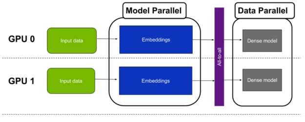
Horovod all-to-all
Moving from the model-parallel to the data-parallel paradigm requires a multi-GPU collective communication operation: All-to-all.
All-to-all is a flexible, collective communication primitive that enables exchange of data between each pair of GPUs. It is required because at the end of the embedding lookup phase, each GPU holds the lookup results for all samples. However, only for a subset of tables (for table-wise split) or a subset of columns (for column-wise split).
Because the all-to-all operation shuffles the data between the GPUs, it is important to note that each GPU holds embedding lookup results for all columns of all tables, but only for a subset of samples. For example, for an eight GPUs scenario, the local batch size after all-to-all is 8x smaller than before all-to-all.
The communication is handled by the Horovod library’s hvd.alltoall function. Under the hood, Horovod calls the NCCL implementation for best performance. It also takes advantage of NVLink if it’s available on your system.
Example of hybrid-parallel training in TensorFlow 2
In this section, I describe a hybrid-parallel training methodology for a 113 billion-parameter recommender system trained in TensorFlow 2. The full source code is available in the NVIDIA Deep Learning Examples repository.
Architecture of Deep Learning Recommendation Model
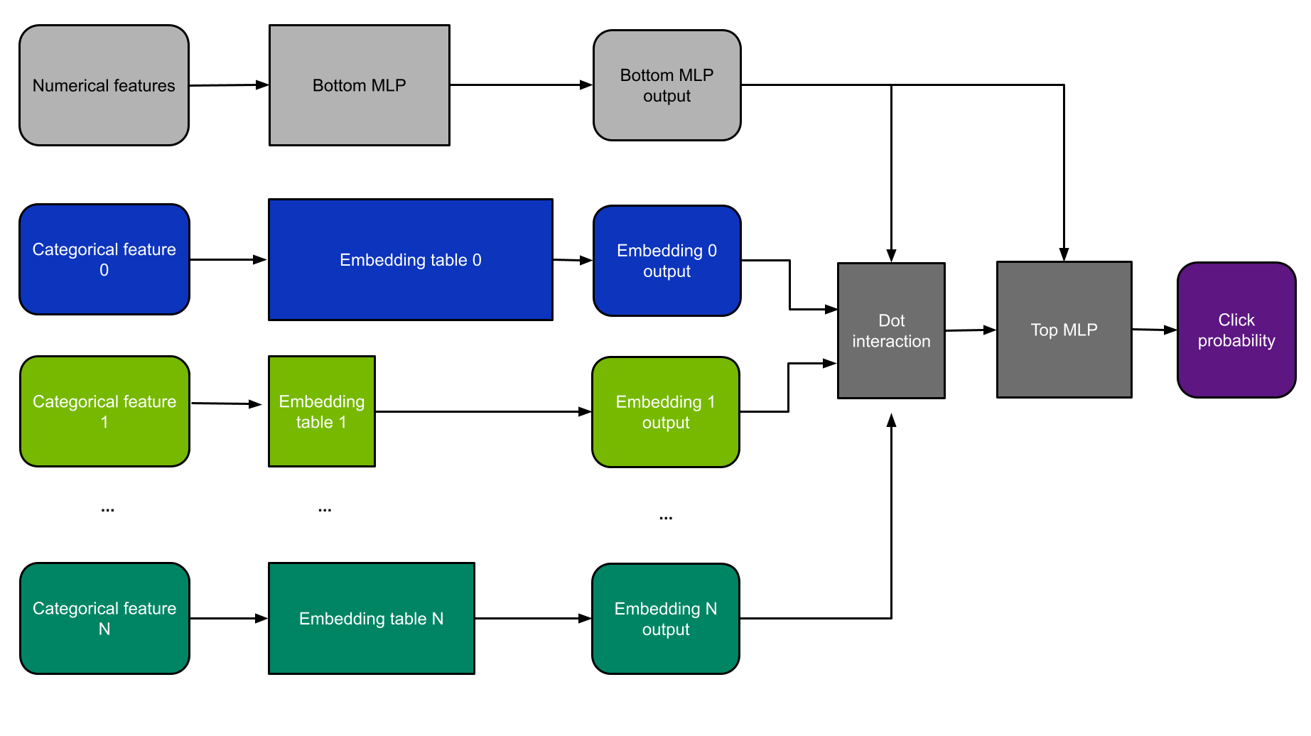
For this example, I use DLRM architecture (Figure 4). DLRM is a class of recommendation models first introduced in the research paper Deep Learning Recommendation Model for Personalization and Recommendation Systems. I chose it because the MLPerf benchmark uses a smaller version of DLRM, and therefore, it is the current industry standard for demonstrating recommender system performance.
DLRM consumes both categorical and numerical features. Categorical features are fed into embedding layers, while numerical features are handled by a small MLP subnetwork.
The results of these layers are then fed into the dot-interaction layer and another MLP. The model is then trained by backpropagation using a binary cross-entropy loss function, and weights are updated according to the Stochastic Gradient Descent (SGD) method.
Modifications to support Wide&Deep models
Although I chose to use DLRM architecture for this example, related models (such as Wide&Deep) can also be supported. This would require the following modifications:
- Add the “wide” part of Wide&Deep, and run it in pure data-parallel mode, completely bypassing the all-to-all.
- Add a second optimizer for the wide part.
- In the deep part, remove the bottom MLP, and pass the numerical features directly to the top MLP.
- Remove the dot-interaction layer.
Criteo dataset
DLRM can be trained on any tabular dataset consisting of numerical and categorical features. For this example, I use the Terabyte Click Logs dataset from Criteo because it is the largest publicly available click-through-rate dataset.
This dataset consists of 26 categorical and 13 numerical variables. Within the unprocessed data, the total number of unique categories is 882 million, of which 292 million is found in the largest feature.
Following the MLPerf recommendation benchmark, you use single precision for the embeddings, with an embedding dimension of 128 for each feature. This means that the total number of parameters is 882M × 128 = 113 billion. The total size of all 26 tables is 113 billion × 4 bytes / 230 = 421 GiB, and the largest table is 139.6 GiB. Because the largest table doesn’t fit into a single GPU, you must use column-wise split mode to slice the tables in pieces and distribute each one across multiple GPUs.
Theoretically, you could implement this for only the few tables that exceed single GPU memory, and use table-wise split for the remainder. However, this would unnecessarily complicate the code without any clear benefit. Therefore, use the column-wise split mode for all tables.
Performance optimizations
To improve training speed, my team implemented the following performance optimizations as shown in the code. These are general tactics that can be applied to other deep learning recommender systems, as well as other deep learning frameworks.
Automatic mixed precision
Mixed precision is the combined use of different numerical precisions in a computational method. For more information about how to enable it, see Mixed precision in the TensorFlow Core documentation. Using mixed precision for this model makes it 23% faster when compared with the default TF32 precision on A100.
Fusing embedding tables of the same width
When several embedding tables have the same vector size–which is the case in DLRM with embedding_dim=128–they can be concatenated along the zero axis. This allows the execution of a single lookup into a large table, instead of multiple lookups into many smaller tables.
Launching one large kernel as opposed to multiple smaller ones is much more efficient. In this example, concatenating the tables results in 39% faster training. For more information, see the NVIDIA/DeepLearningExamples/blob/master/TensorFlow2/Recommendation/DLRM GitHub repo.
XLA
My team used the TensorFlow Accelerated Linear Algebra (XLA) compiler to improve performance. For this particular use case, applying XLA yields a 3.36x speedup compared to not using it. This value was achieved with all other optimizations being turned on: AMP, concatenated embedding, and so on.
Broadcasting dataloader
Running a piece of each embedding table on every GPU means that each GPU must access each feature of every training sample. Loading and parsing all this input data separately in each process is inefficient and can result in major bottlenecks. I addressed this by loading the input data only on the first worker and broadcasting it over NVLink to the others. This provides a 32% speedup.
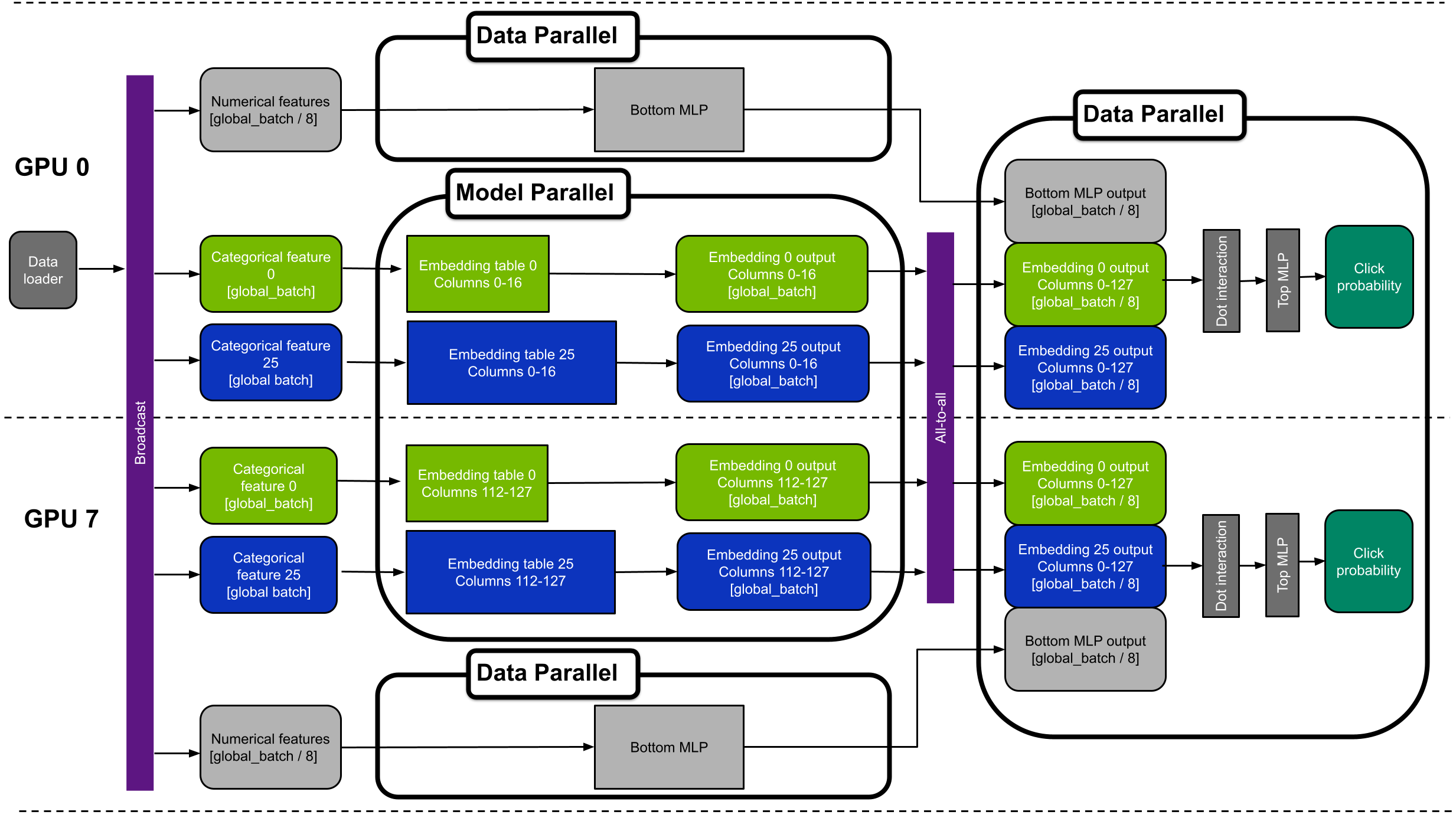
Putting it all together
Figure 5 shows an example device placement for the hybrid-parallel DLRM with eight GPUs. The diagram shows GPUs 0 and 7. For simplicity, it only shows categorical features 0 and 25.
Alternative approach: store the large embeddings on CPU
A simple alternative for storing large embedding matrices is to put them into host memory. Small embedding tables and compute-intensive layers can still be placed on GPU for best performance. Although much simpler, this approach is also slower when compared to keeping all variables on GPU.
There are two fundamental reasons for this:
- Embedding lookup is a memory-bound operation. CPU memory is much slower than GPU memory. The total memory bandwidth is 409.6 GB/s for a dual-socket AMD Epyc 7742 compared to 2 TB/s for a single A100-80GB GPU and 16 TB/s for a total of 8 A100-80GB GPUs.
- Exchanging data between GPUs is significantly faster than between the CPU and GPU. This is because the PCIe link between connecting the CPU to GPU can become a bottleneck.
When using the CPU to store the embeddings, the transfers between the CPU and GPU must first pass through the PCIe interface providing 31.5 GB/sec of bandwidth. Conversely, in the hybrid-parallel paradigm, the results of the embedding lookups travel instead through NVSwitch fabric between the GPUs. DGX A100 uses second-generation NVSwitch technology, enabling 600 GB/sec of peak GPU-to-GPU communication.
Despite these slowdowns, this alternative approach is still much faster than running the entire network on the CPU alone.
Benchmark results
The following table shows benchmark results for training the 113B-parameter DLRM model. It compares three hardware setups: CPU only, a single GPU that uses CPU memory for the largest embedding tables, and a hybrid-parallel approach using the full DGX A100-80GB.
| Hardware | Throughput [samples/second] | Speedup over CPU |
| 2xAMD EPYC 7742 | 17.7k | 1x |
| A100-80GB + 2xAMD EPYC 7742(large embeddings on CPU) | 768k | 43x |
| DGX A100 (8xA100-80GB) (hybrid parallel) | 11.9M | 672x |
Comparing the first two rows, you can see that complementing two CPUs with a single A100 GPU yields a 43x increase in throughput. This occurs because the GPU is highly suitable for running compute-intensive linear layers and the smaller embedding layers that fit into its 80-GB memory.
Moreover, using the full DGX A100 with eight GPUs is 15.5x faster than training on a single A100 GPU. The DGX A100 enables you to fit the entire model into the GPU memory and removes the need for costly device-to-host and host-to-device transfers.
Overall, the DGX A100 solves this task 672x faster than a dual-socket CPU system.
Conclusion
In this post, I introduced the idea of using hybrid-parallelism to train large recommender systems. The results of this test showed that DGX A100 is an excellent tool for training recommender systems with over 100 billion parameters in TensorFlow 2. It achieved a 672x speedup over a dual-socket CPU.
High memory bandwidth and fast GPU-to-GPU communication make it possible to train recommenders quickly. As a result, you experience shorter training times when compared to using only CPU servers. This lowers training costs while simultaneously enabling faster experimentation for practitioners.