
 Researchers at NVIDIA have developed methods to improve and accelerate sampling from diffusion models, a novel and powerful class of generative models.
This is part of a series on how NVIDIA researchers have developed methods to improve and accelerate sampling from diffusion models, a novel and powerful class of generative models. Part 2 covers three new techniques for overcoming the slow sampling challenge in diffusion models.
Generative models are a class of machine learning methods that learn a representation of the data they are trained on and model the data itself. They are typically based on deep neural networks. In contrast, discriminative models usually predict separate quantities given the data.
Generative models allow you to synthesize novel data that is different from the real data but still looks just as realistic. A designer could train a generative model on images of cars and then let the resulting generative AI computationally dream up novel cars with different looks, accelerating the artistic prototyping process.
Deep generative learning has become an important research area in the machine learning community and has many relevant applications. Generative models are widely used for image synthesis and various image-processing tasks, such as editing, inpainting, colorization, deblurring, and superresolution.
Generative models have the potential to streamline the workflow of photographers and digital artists and enable new levels of creativity. Similarly, they might allow content creators to efficiently generate virtual 3D content for games, animated movies, or the metaverse.
Deep learning-based speech and language synthesis have already found their way into consumer products. Fields such as medicine and healthcare may also benefit from generative models, such as methods that generate molecular drug candidates to fight disease.
The data representations learned by the neural networks of generative models, as well as the synthesized data, can often be used for training and fine-tuning other downstream machine learning models for different tasks, especially when labeled data is scarce.
Generative learning trilemma
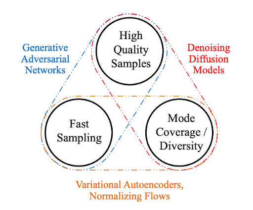
For a wide adoption in real-world applications, generative models should ideally satisfy the following key requirements:
- High-quality sampling: Many applications, especially those directly interacting with users, require high generation quality. For example, in speech generation, poor speech quality is difficult to understand. Similarly, in image modeling, the desired outputs are visually indistinguishable from natural images.
- Mode coverage and sample diversity: If the training data contains a complex or large amount of diversity, a good generative model should successfully capture such diversity without sacrificing generation quality.
- Fast and computationally inexpensive sampling: Many interactive applications require fast generation, such as real-time image editing.
While most current methods in deep generative learning focus on high-quality generation, the second and third requirements are highly important as well.
A faithful representation of the data’s diversity is crucial to avoid missing minority modes in the data distribution. This helps reduce undesired biases in the learned models.
On the other hand, in many applications, the long tails of the data distribution are particularly interesting. For instance, in traffic modeling, it is precisely the rare scenarios that are of interest, those that correspond to dangerous driving or accidents.
Reducing computational complexity and sampling time not only enables interactive, real-time applications. It also lessens the environmental footprint of running the expensive deep neural networks that underlie generative models by decreasing the overall power usage required for generation.
In this post, we identify the challenge imposed by these three requirements as the generative learning trilemma as existing methods usually make trade-offs and cannot satisfy all requirements simultaneously.
Generative learning with diffusion models
Recently, diffusion models have emerged as a powerful class of generative learning methods. These models,, also known as denoising diffusion models or score-based generative models, demonstrate surprisingly high sample quality, often outperforming generative adversarial networks. They also feature strong mode coverage and sample diversity.
Diffusion models have already been applied to a variety of generation tasks, such as image, speech, 3D shape, and graph synthesis.
Diffusion models consist of two processes: forward diffusion and parametrized reverse.
A forward diffusion process maps data to noise by gradually perturbing the input data. This is formally achieved by a simple stochastic process that starts from a data sample and iteratively generates noisier samples using a simple Gaussian diffusion kernel. That is to say, at each step of this process, Gaussian noise is incrementally added to the data.
The second process is a parametrized reverse process that undoes the forward diffusion and performs iterative denoising. This process represents data synthesis and is trained to generate data by converting random noise into realistic data. It is also formally defined as a stochastic process, which iteratively denoises input images using trainable deep neural networks.
Both the forward and reverse processes often use thousands of steps for gradual noise injection and during generation for denoising.
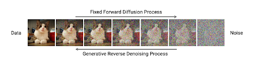
Figure 2 shows that, in diffusion models, a fixed forward process gradually perturbs the data in a stepwise fashion towards fully random noise. A parametrized reverse process is learned to perform iterative denoising and to generate data, such as images, from noise.
Formally, denoting a data point such as an image by 


At each step, 


The reverse generative process is similarly defined in reverse order by:

In this formula, the denoising distribution 

These processes are described in terms of discretized diffusion and denoising steps, indexed by a parameter
Continuous-time diffusion models
However, you can also study diffusion models in the limit of an infinite number of infinitely small time steps. This leads to continuous-time diffusion models where time flows continuously. In this case, the forward and reverse processes can be described using stochastic differential equations (SDEs).
A fixed forward SDE smoothly transforms a data sample into random noise. One option for such an SDE is as follows:

As before, 


Although discrete-time and continuous-time diffusion models may seem different, they share an almost identical generative process. In fact, it is easy to show that discrete-time diffusion models are special discretizations of continuous-time models.
Working with continuous-time diffusion models in practice is essentially a lot easier:
- They are more generic and can be converted to discrete-time models using simple discretizations of time.
- They are described using SDEs, which are well-studied in various scientific domains.
- The generative SDEs can be solved using off-the-shelf numerical SDE solvers.
- They can be converted to related ordinary differential equations (ODEs), which are also well-studied and easy to work with.
As mentioned earlier, diffusion models generate samples by following the reverse diffusion process that maps a simple base distribution, typically Gaussian, to the complex data distribution. This mapping, in continuous-time diffusion models represented by the generative SDE, is often complex due to the neural network approximating the score function.
Solving it with numerical integration techniques can require 1000s of calls to deep neural networks for sample generation. Because of this, diffusion models are often slow at sample generation, requiring minutes or even hours of computation time. This stands in stark contrast to competing techniques such as generative adversarial networks (GANs), which generate samples using only one call to a neural network.
Summary
Although diffusion models achieve high sample quality and diversity, they unfortunately fall short in sampling speed. This limits the wide adoption of diffusion models for practical real-world applications and has led to an active area of research on accelerated sampling from these models. In Part 2, we review three techniques developed at NVIDIA for overcoming the main limitation of diffusion models.
To learn more about the research that NVIDIA is advancing, see NVIDIA Research.
For more information about diffusion models, see the following resources:
- Score-based Generative Modeling in Latent Space paper
- Project page: /LSGM GitHub repo
- Score-Based Generative Modeling with Critically-Damped Langevin Diffusion paper
- Project page: /CLD-SGM GitHub repo
- Tackling the Generative Learning Trilemma with Denoising Diffusion GANs paper
- Project page: /denoising-diffusion-gan GitHub repo