
|
submitted by /u/7NoteDancing [visit reddit] [comments] |
Categories
Is anyone interested in this project?

 DataBloom
|
|
submitted by /u/7NoteDancing [visit reddit] [comments] |

|
How do I fix this error message? Tried googling it with no luck. submitted by /u/Ok_Wish4469 |
 We present lessons learned from refactoring a Fortran application to use modern do concurrent loops in place of OpenACC for GPU acceleration.
This is the fourth post in the Standard Parallel Programming series, which aims to instruct developers on the advantages of using parallelism in standard languages for accelerated computing:
Standard languages have begun adding features that compilers can use for accelerated GPU and CPU parallel programming, for instance, do concurrent loops and array math intrinsics in Fortran.
Using standard language features has many advantages to offer, the chief advantage being future-proofness. As Fortran’s do concurrent is a standard language feature, the chances of support being lost in the future is slim.
This feature is also relatively simple to use in initial code development and it adds portability and parallelism. Using do concurrent for initial code development has the mental advantage of encouraging you to think about parallelism from the start as you write and implement loops.
For initial code development, do concurrent is a great way to add GPU support without having to learn directives. However, even code that has already been GPU-accelerated through the use of directives like OpenACC and OpenMP can benefit from refactoring to standard parallelism for the following reasons:
POT3D is a Fortran code that computes potential field solutions to approximate the solar coronal magnetic field using surface field observations as input. It continues to be used for numerous studies of coronal structure and dynamics.
The code is highly parallelized using MPI and is GPU-accelerated using MPI with OpenACC. It is open source and available on GitHub. It is also a part of the SpecHPC 2021 Benchmark Suites.
We recently refactored another code example with do concurrent at WACCPD 2021. The results showed that you could replace directives with do concurrent without losing performance on multicore CPUs and GPUs. However, that code was somewhat simple in that there is no MPI.
Now, we want to explore replacing directives in more complicated code. POT3D contains nontrivial features for standard Fortran parallelism to handle: reductions, atomics, CUDA-aware MPI, and local stack arrays. We want to see if do concurrent can replace directives and retain the same performance.
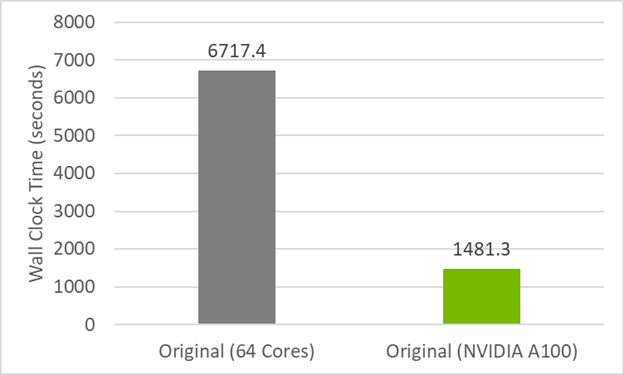
To establish a performance baseline for refactoring the code to do concurrent, first review the initial timings of the original code in Figure 1. The CPU result was run on 64 MPI ranks (32 per socket) on a dual-socket AMD EPYC 7742 server, while the GPU result was run on one MPI rank on an NVIDIA A100 (40GB). The GPU code relies on data movement directives for data transfers (we do not use managed memory here) and is compiled with -acc=gpu -gpu=cc80,cuda11.5. The runtimes are an average over four runs.
The following highlighted text shows the number of lines of code and directives for the current version of the code. You can see that there are 80 directives, but we hope to reduce this number by refactoring with do concurrent.
| POT3D (Original) | |
| Fortran | 3,487 |
| Comments | 3,452 |
| OpenACC Directives | 80 |
| Total | 7,019 |
Here are some examples of do concurrent compared to OpenACC from the code POT3D, such as a triple-nested OpenACC parallelized loop:
!$acc enter data copyin(phi,dr_i)
!$acc enter data create(br)
…
!$acc parallel loop default(present) collapse(3) async(1)
do k=1,np
 do j=1,nt
  do i=1,nrm1
   br(i,j,k)=(phi(i+1,j,k)-phi(i,j,k))*dr_i(i)
  enddo
 enddo
enddo
…
!$acc wait
!$acc exit data delete(phi,dr_i,br)
As mentioned earlier, this OpenACC code is compiled with the flag -acc=gpu -gpu=cc80,cuda11.5 to run on an NVIDIA GPU.
You can parallelize this same loop with do concurrent and rely on NVIDIA CUDA Unified Memory for data movement instead of directives. This results in the following code:
do concurrent (k=1:np,j=1:nt,i=1:nrm1)
 br(i,j,k)=(phi(i+1,j,k)-phi(i,j,k ))*dr_i(i)
enddo
As you can see, the loop has been condensed from 12 lines to three, and CPU portability and GPU parallelism are retained with the nvfortran compiler from the NVIDIA HPC SDK.
This reduction in the number of lines is thanks to collapsing multiple loops into one loop and relying on managed memory, which removes all data movement directives. Compile this code for the GPU with -stdpar=gpu -gpu=cc80,cuda11.5.
For nvfortran, activating standard parallelism (-stdpar=gpu) automatically activates managed memory. To use OpenACC directives to control data movement along with do concurrent, use the following flags: -acc=gpu -gpu=nomanaged.
The nvfortran implementation of do concurrent also allows for locality of variables to be defined:
do concurrent (k=1:N, j(i)>0) local(M) shared(J,K)
 M = mod(K(i), J(i))
 K(i) = K(i)- M
enddo
This may be necessary for some code. For POT3D, the default locality of variables performs as needed. The default locality is the same as OpenACC with nvfortran.
Replacing all the OpenACC loops with do concurrent and relying on managed memory for data movement leads you to code with zero directives and fewer lines. We removed 80 directives and 66 lines of Fortran.
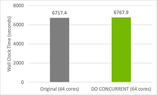
Figure 2 shows that this do concurrent version of the code has nearly the same performance on the CPU as the original GitHub code. This means that you haven’t broken CPU compatibility by using do concurrent. Instead, multi-core parallelism has also been added, which can be used by compiling with the flag -stdpar=multicore.
Unlike the case of the CPU, to be able to run POT3D on a GPU, you must add a couple of directives.
First, to take advantage of multiple GPU with MPI, you need a directive to specify the GPU device number. Otherwise, all MPI ranks would use the same GPU.
!$acc set device_num(mpi_shared_rank_num)In this example, mpi_shared_rank_num is the MPI rank within a node. It’s assumed that the code is launched such that the number of MPI ranks per node is the same as the number of GPUs per node. This can also be accomplished by setting CUDA_VISIBLE_DEVICES for each MPI rank, but we prefer doing this programmatically.
When using managed memory with multiple GPUs, make sure that the device selection (such as !$acc set device_num(N)) is done before any data is allocated. Otherwise, an additional CUDA context is created, introducing additional overhead.
Currently, the nvfortran compiler does not support array reductions on concurrent loops, which are required in two places in the code. Fortunately, an OpenACC atomic directive can be used in place of an array reduction:
do concurrent (k=2:npm1,i=1:nr)
!$acc atomic
 sum0(i)=sum0(i)+x(i,2,k)*dph(k )*pl_i
enddo
After adding this directive, change the compiler options to enable OpenACC explicitly by using -stdpar=gpu -acc=gpu -gpu=cc80,cuda11.5. This allows you to use only three OpenACC directives. This is the closest this code can come to not having directives at this time.
All the data movement directives are unnecessary, since CUDA managed memory is used for all data structures. Table 2 shows the number of directives and lines of code needed for this version of POT3D.
| POT3D (Original) | POT3D (Do Concurrent) | Difference | |
| Fortran | 3487 | 3421 | (-66) |
| Comments | 3452 | 3448 | (-4) |
| OpenACC Directives | 80 | 3 | (-77) |
| Total | 7019 | 6872 | (-147) |
For the reduction loops in POT3D, you relied on implicit reductions, but that may not always work. Recently, nvfortran has added the upcoming Fortran 202X reduce clause, which can be used on reduction loops as follows:
do concurrent (k=1:N) reduce(+:cgdot)
 cgdot=cgdot+x(i)*y(i)
enddoYou’ve developed code with the minimal number of OpenACC directives and do concurrent that relies on managed memory for data movement. This is the closest directive-free code that you can have at this time.
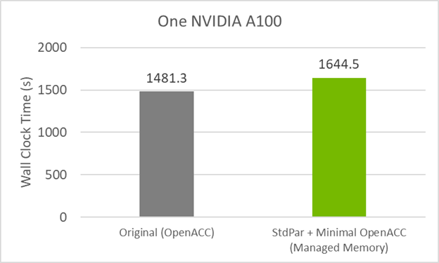
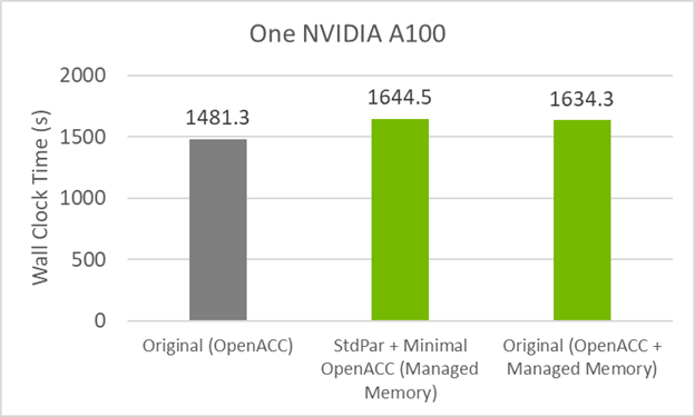
Figure 3 shows that this code version takes a small performance hit of ~10% when compared to the original OpenACC GPU code. The cause of this could be do concurrent, managed memory, or a combination.
To see if managed memory causes the small performance hit, compile the original GitHub code with managed memory turned on. This is done by using the compile flag -gpu=managed in addition to the standard OpenACC flags used before for the GPU.
Figure 4 shows that the GitHub code now performs similar to the minimum directives code with managed memory. This means that the culprit for the small performance loss is unified memory.
To regain the performance of the original code with the minimal directives code, you must add the data movement directives back in. This mixture of do concurrent and data movement directives would look like the following code example:
!$acc enter data copyin(phi,dr_i)
!$acc enter data create(br)
do concurrent (k=1:np,j=1:nt,i=1:nrm1)
 br(i,j,k)=(phi(i+1,j,k)-phi(i,j,k ))*dr_i(i)
enddo
!$acc exit data delete(phi,dr_i,br)
This results in the code having 41 directives, with 38 being responsible for data movement. To compile the code and rely on the data movement directives, run the following command:
-stdpar=gpu -acc=gpu -gpu=cc80,cuda11.5,nomanaged
nomanaged turns off managed memory and -acc=gpu turns on the directive recognition.
Figure 5 shows that there is nearly the same performance as the original GitHub code. This code has 50% fewer directives than the original code and gives the same performance!
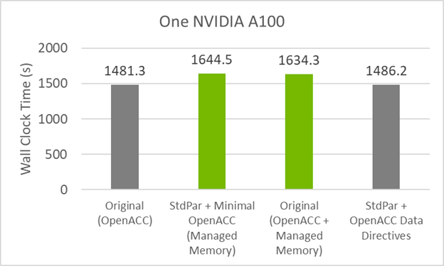
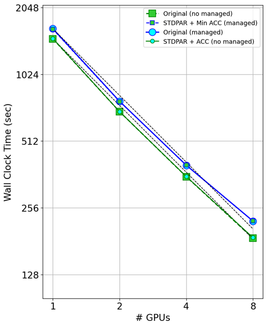
Figure 7 shows the timing results using multiple GPUs. The primary takeaway is that do concurrent works with MPI over multiple GPUs.
Looking at the codes with managed memory turned on (blue lines), you can see that the original code and the minimal directives code gave nearly the same performance as multiple GPUs were used.
Looking at the codes with managed memory turned off (green lines), you can again see the same scaling between the original GitHub code and the do concurrent version of the code. This indicates that do concurrent works with MPI and has no impact on the scaling you should see.
What you might also notice is that managed memory causes an overhead as the GPUs are scaled. The managed memory runs (blue lines) and data directive lines (green lines) are parallel to each other, meaning the overhead scales with the number of GPUs.
You may be wondering, “Standard Fortran sounds too good to be true, what is the catch?”
Fortran standard parallel programming enables cleaner looking code and increases the future proofness of your code by relying on ISO language standards. Using the latest nvfortran compiler, you gain all the benefits mentioned earlier.
Although you lose the current GCC OpenACC/MP GPU support when you transition to do concurrent, we expect to gain more GPU support in the future as other vendors add support of do concurrent on GPUs. Given the track record of ISO language standards, we believe that this support will come.
Using do concurrent does currently come with a small number of limitations, namely the lack of support for atomics, device selection, asynchrony, or optimizing data movement. As we have shown, however, each of these limitations can be easily worked around using compiler directives. Far fewer directives are required thanks to the native parallel language features in Fortran.
Ready to get started? Download the free NVIDIA HPC SDK, and start testing! If you are also interested in more details on our findings, see the From Directives to DO CONCURRENT: A Case Study in Standard Parallelism GTC session. For more information about standard language parallelism, see Developing Accelerated Code with Standard Language Parallelism.
This work was supported by the National Science Foundation, NASA, and the Air Force Office of Scientific Research. Computational resources were provided by the Computational Science Resource Center at San Diego State University.
 Learn how RAPIDS cuDF accelerates data science with the help of GPUDirect Storage. Dive into the techniques that minimize the time to upload data to the GPU
If you work in data analytics, you know that data ingest is often the bottleneck of data preprocessing workflows. Getting data from storage and decoding it can often be one of the most time-consuming steps in the workflow because of the data volume and the complexity of commonly used formats. Optimizing data ingest can greatly reduce this bottleneck for data scientists working on large data sets.
RAPIDS cuDF greatly speeds up data decode by implementing CUDA-accelerated readers for prevalent formats in data science.
In addition, Magnum IO GPUDirect Storage (GDS) enables cuDF to speed up I/O by loading the data directly from storage into the device (GPU) memory. By providing a direct data path across the PCIe bus between the GPU and compatible storage (for example, Non-Volatile Memory Express (NVMe) drive), GDS can enable up to 3–4x higher cuDF read throughput, with an average of 30–50% higher throughput across a variety of data profiles.
In this post, we provide an overview of GPUDirect Storage and how it’s integrated into cuDF. We introduce the suite of benchmarks that we used to evaluate I/O performance. Then, we walk through the techniques that cuDF implements to optimize GDS reads. We conclude with the benchmark results and identify cases where use of GDS is the most beneficial for cuDF.
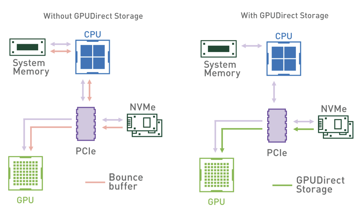
GPUDirect Storage is a new technology that enables direct data transfer between local or remote storage (as a block device or through file systems interface) and GPU memory.
In other words, a direct memory access (DMA) engine can now quickly move data on a direct path from the storage to GPU memory, without increasing latency and burdening the CPU with extra copying through a bounce buffer.
Figure 1 shows the data flow patterns without and with GDS. When using the system memory bounce buffer, throughput is bottlenecked by the bandwidth from system memory to GPUs. On systems with multiple GPUs and NVMe drives, this bottleneck is even more pronounced.
However, with the ability to directly interface GPUs with storage devices, the intermediary CPU is taken out of the data path, and all CPU resources can be used for feature engineering or other preprocessing tasks.
The GDS cuFile library enables applications and frameworks to leverage GDS technology to increase bandwidth and achieve lower latency. cuFile is available as part of CUDA Toolkit since version 11.4.
To increase the end-to-end read throughput, cuDF uses the cuFile APIs in its data ingest interfaces, like read_parquet and read_orc. As cuDF performs nearly all parsing on the GPU, most of the data is not needed in system memory and can be directly transferred to GPU memory.
As a result, only the metadata portion of input files is accessed by the CPU, and the metadata constitutes only a small part of the total file size. This permits the cuDF data ingest API to make efficient use of GDS technology.
Since cuDF 22.02, we have enabled the use of GDS by default. If you have cuFile installed and request to read data from a supported storage location, cuDF automatically performs direct reads through the cuFile API. If GDS is not applicable to the input file, or if the user disables GDS, data follows the bounce buffer path and is copied through a paged system memory buffer.
In response to the diversity of data science datasets, we assembled a benchmark suite that targets key data and file properties. Previous examples of I/O benchmarking used data samples such as the New York Taxi trip record, the Yelp reviews dataset, or Zillow housing data to represent general use cases. However, we discovered that benchmarking specific combinations of data and file properties have been crucial for performance analysis and troubleshooting.
Table 1 shows the parameters that we varied in our benchmarks for binary formats. We generated pseudo-random data across the range of supported data types and collected benchmarks for each group of related types. We also independently varied the run-length and cardinality of the data to exercise run-length encoding and dictionary encoding of the target formats.
Finally, we varied the compression type in the generated files, for all values of the properties preceding. We currently support two options: Use Snappy or keep the data uncompressed.
| Data Property | Description |
| File format | Parquet, ORC |
| Data type | Integer (signed and unsigned) Float (32-, 64-bit) String (90% ASCII, 10% Unicode) Timestamp (day, s, ms, us, ns) Decimal (32-, 64-, 128-bit) List (nesting depth 2, int32 elements) |
| Run-length | Average data value repetition (1x or 32x) |
| Cardinality | Unique data values (unlimited or 1000) |
| Compression | Lossless compression type (Snappy or none) |
With all of the properties that change independently, we have a large number of varied cases: 48 cases for each file format (ORC and Parquet). To ensure fair comparison between cases, we targeted a fixed in-memory dataframe size and column count, with a default size of 512 MiB. For the purpose of this post, we introduced an additional parameter to control the target in-memory dataframe size from 64 to 4,096 MiB.
The full cuDF benchmark suite is available in the open-source cuDF repository. To focus on the impact of I/O, this post only includes the inputs benchmarks in cuDF rather than reader options or row/column selection benchmarks.
Data in formats like ORC and Parquet are stored in independent chunks, which we read in separate operations. We found that the read bandwidth is not saturated when these operations are performed in a single thread, leading to suboptimal performance regardless of GDS use.
Issuing multiple GDS read calls in parallel enables overlapping of multiple storage-to-GPU copies, raising the throughput and potentially saturating the read bandwidth. As of version 1.2.1.4, cuFile calls are synchronous, so parallelism requires multithreading from downstream users.
As we did not control the file layout and number of data chunks, creating a separate thread for each read operation could have generated an excessive number of threads, leading to a performance overhead. On the other hand, if we only had a few large read calls, we might not have had enough threads to effectively saturate the read bandwidth of the storage hardware.
To control the level of parallelism, we used a thread pool and sliced larger read calls into smaller reads that could be performed in parallel.
When we begin reading a file using GDS, we create a data ingest pipeline based on the thread-pool work of Barak Shoshany from Brock University. As Figure 2 shows, we split each file read operation (read_async call) in the cuDF reader into cuFile calls of fixed size, except for, in most cases, the last slice.
Instead of directly calling cuFile to read the data, a task is created for each slice and placed in a queue. The read_async call returns a task that waits for all of the sliced tasks to be completed. Callers can perform other work and wait on the aggregate task after the requested data is required to continue. When available, threads from the pool dequeue the tasks and make the synchronous cuFile calls.
Upon completion, a thread sets the task as completed and becomes available to execute the next task in the queue. As most tasks read the same amount of data, cuFile reads are effectively load-balanced between the threads. After all tasks from a given read_async call are completed, the aggregate task is complete and the caller code can continue, as the requested data range has been uploaded to the GPU memory.
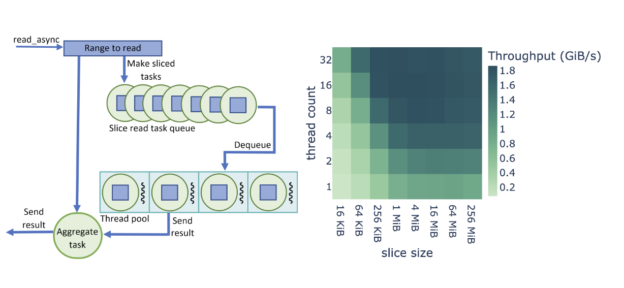
The size of the thread pool and the read slices greatly impacts the number of GDS read calls executed at the same time. To maximize throughput, we experimented with a range of different values for these parameters and identified the configuration that gives the highest throughput.
Figure 2 shows a performance optimization study on cuDF+GDS data ingest with tunable parameters of thread count and slice size. For this study, we defined the end-to-end read throughput as the binary format file size divided by the total ingest time (I/O plus parsing and decode).
The throughput shown in Figure 2 is averaged over the entire benchmark suite and based on a dataframe size of 512 MiB. We found that Parquet and ORC binary formats share the same optimization behavior across the parameter range, also shown in Figure 2. Small slice sizes cause higher overhead due to the large number of read tasks, and large slice sizes lead to poor utilization of the thread pool.
In addition, lower thread counts do not provide enough parallelism to saturate the NVMe read bandwidth, and higher thread counts lead to thread overhead. We discovered that the highest end-to-end read throughput was for 8-32 threads and 1-16 MiB slice size.
Depending on the use case, you may find optimal performance with different values. This is why, as of 22.04, the default thread pool size of 16 and slice size of 4 MiB are configurable through environment variables, as described in GPUDirect Storage Integration.
We evaluated the effect that GDS use had on the performance of a few cuDF data ingest APIs using the benchmark suite described earlier. To isolate the impact of GDS, we ran the same set of benchmarks with default configuration (uses GDS) and with GDS manually disabled through an environment variable.
For accurate I/O benchmarking with cuDF benchmarks, file system caches must be cleared before each new read operation. Benchmarks measure the total time to execute a read_orc or read_parquet call (read time) and these are the values we used for comparison. GDS speedup was computed for each benchmark case file as the read time through the bounce buffer divided by the total ingest time through the direct data path.
For the GDS performance comparison, we used a NVIDIA DGX-2 with V100 GPUs and NVMe SSDs connected in a RAID 0 configuration. All benchmarks use a single GPU and read from a single RAID 0 of two 3.84-TB NVMe SSDs.
Figure 3 shows the GDS speedup for a variety of files with in-memory dataframe size of 4,096 MiB. We observed that the performance improvement varies widely, between modest 10% and impressive 270% increase over the host path.
Some of the variance is due to differences in the data decode. For example, list types show smaller speedups due to the higher parsing complexity, and decimal types in ORC show smaller speedups due to overhead in fixed point decoding compared to Parquet.
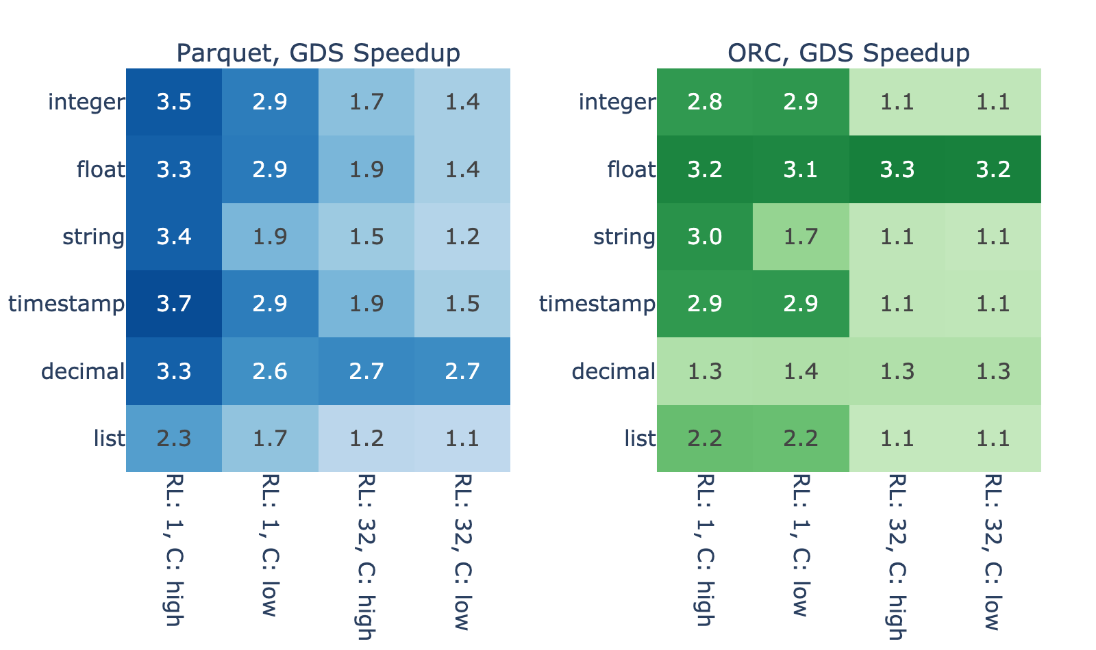
However, the decode process cannot account for the majority of variance in the results. With high correlation between the result for ORC and Parquet, you can reasonably suspect that properties like run-length and cardinality play a major role. Both properties affect how well data can be compressed/encoded, so here’s how the file size relates to these properties and, by proxy, to the GDS speedup.
Figure 4 shows the extent in which intrinsic properties of the data impact the binary file size needed to store a fixed in-memory data size. For 4,096 MiB of in-memory data, file sizes range from 0.1 to 5.8 GB across the benchmarks cases without Snappy compression. As expected, the largest file sizes generally correspond to shorter run-length and higher cardinality because data with this profile is difficult to efficiently encode.
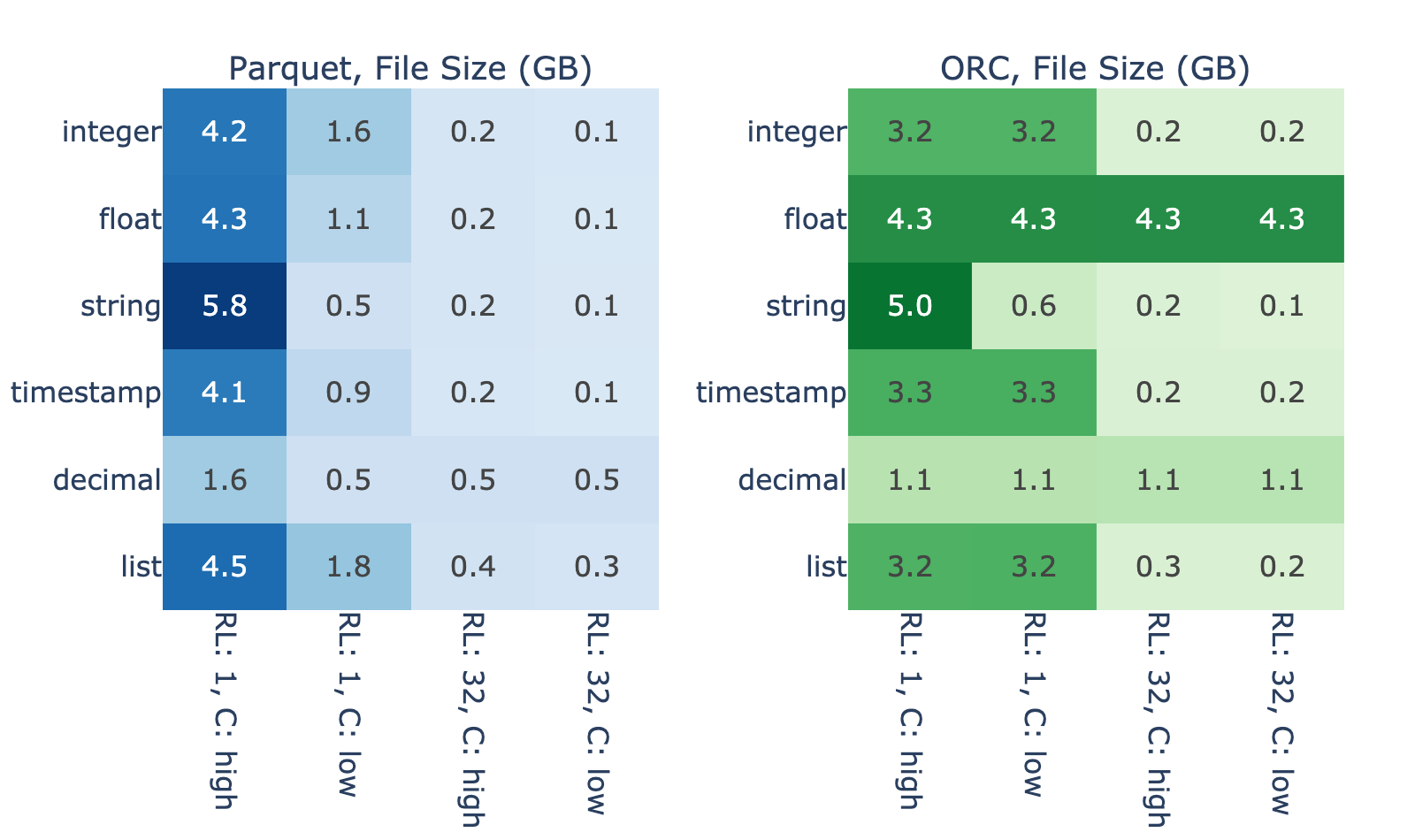
Figures 3 and 4 show strong correlation between file size and the magnitude of GDS performance benefit. We hypothesize that this is because, when reading an efficiently encoded file, I/O takes less time compared to decode so there’s little room for improvement from GDS. On the other hand, the results show that reading of files that encode poorly is bottlenecked on the I/O.
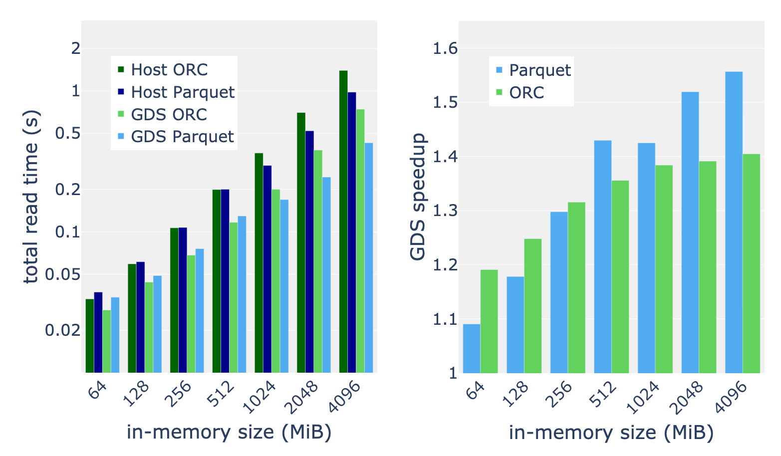
We applied the full benchmark suite described in Table 1 to inputs with in-memory sizes in the range of 64 to 4,096 MiB. Taking the mean speedup over the benchmark suite, we discovered that speedup from GDS generally increases with the data size. We measure consistent 30-50% speedup for 512 MiB and greater in-memory data sizes. For the largest datasets, we found that the Parquet reader benefits more from GDS than the ORC reader.
GPUDirect Storage provides a direct data path to the GPU, reducing latency and increasing throughput for I/O operations. RAPIDS cuDF leverages GDS in its data ingest APIs to unlock the full read bandwidth of your storage hardware.
GDS enables you to speed up cuDF data ingest workloads up to 3x, significantly improving the end-to-end performance of your workflows.
If you have not tried out cuDF for your data processing workloads, we encourage you to test our latest 22.04 release. We provide Docker containers for our releases as well as our nightly builds. Conda packages are also available to make testing and deployment easier. If you want to get started with RAPIDS cuDF, you can do so.
If you are already using cuDF, we encourage you to give GPUDirect Storage a try. It is easier than ever to take advantage of high capacity and high-performance NVMe drives. If you already have the hardware, you are a few configuration steps away from unlocking peak performance in data ingest. Stay tuned for upcoming releases of cuDF.
For more information about storage I/O acceleration, see the following resources:
SANTA CLARA, Calif., May 27, 2022 — NVIDIA today announced that it recently became aware of an unsolicited “mini-tender” offer by Tutanota LLC to purchase up to 215,000 …
 This post highlights helpful new cuDF features that allow you to think about a single row of data and write code faster.
Over the past few releases, the NVIDIA cuDF team has added several new features to user-defined functions (UDFs) that can streamline the development process while improving overall performance. In this post, I walk through the new UDF enhancements and show how you can take advantage of them within your own applications:
Series.apply API and how to use itDataFrame.apply API and how to write a UDF in terms of “rows”If you’re not familiar with pandas, series apply is the main entry point used for mapping an arbitrary Python function onto a single series of data. For example, you might want to convert temperature in Celsius to Fahrenheit using a formula already written as a Python function.
Here is a quick refresher followed by the output of running this code:
Viewer requires iframe.
Technically, you can write any valid Python code within the function f and pandas runs the function in a loop over the series. This makes apply extremely flexible in the context of pandas, as any UDF can be successfully applied as long as it can successfully handle all of the input data—even UDFs that rely on external libraries or ones that expect or return arbitrary Python objects.
But, this flexibility comes at the cost of performance. Running a Python function in a long loop is not known for being an efficient strategy for a variety of reasons (for example, Python being interpreted from the outset). As a result, this performance constraint can be frustrating if your UDFs are simpler, such as those composed of purely mathematical operations on scalar values.
Luckily, these use cases are what cuDF was built for. Recent cuDF improvements within the scope of UDFs have motivated the introduction of the equivalent apply API:
If you are familiar with pandas, you can produce the same results as you did using pandas for numeric values. The only notable difference is that the resulting data is always a cuDF dtype and not an object, which is usually the case in pandas.
The function f can contain any Python UDF that is composed of pure math or Python operations. cuDF deduces an appropriate return dtype based on the inspection of the function through Numba and compiles and runs an equivalent function on the GPU.
Functions can also be written to accept an arbitrary number of scalar arguments. In the following code example, you can see that args= is supported:
While there are other ways of accomplishing the same goal in cuDF using custom kernels and other methods, this method of writing UDFs helps to abstract the GPU away from the process, which can cut down on development time for data scientists working on fast-paced, real-world projects.
So far, I’ve covered only the case of Series-based data. That is, I’ve shown you how to write a UDF with a single input and output. Many use cases require multi-column input, however, and this requires slightly different thinking.
UDFs that expect multiple columns as input and produce a single column as output are the set of functions supported by the pandas DataFrame apply API.
In these cases, the first function argument represents a row of data rather than just one value from a single input column. By row, I mean some kind of data structure that is keyable to obtain values, where the keys are the column names and the values are the scalars corresponding to the values of those columns in that row. It is conceptually what you get when you use iloc in pandas:
The following code example shows how you would write and use a UDF in pandas that consumes this kind of row object:
cuDF now enables you to do the exact thing without rewriting your UDF.
When applying these functions, it is important to note that even though the cuDF API expects you to write the functions in terms of rows, no rows are actually involved when it comes to the execution of this function.
cuDF avoids the use of a for-loop and instead executes CUDA kernels that “pretend” rows of data exist. With a little magic, Numba knows how to write a proper kernel to get the same result as pandas. Because there is no loop, you should see higher performance when executing functions through this API.
Historically, UDFs in cuDF have not provided full support for missing values. This is due to architectural choices inside cuDF that relate to the way cuDF records which elements are null, specifically its use of a null mask to conserve memory.
The looping design of pandas apply APIs just works if the data contains null values. If a null is encountered in the data, the UDF receives the special value pd.NA. As a result, if the special value does not trigger an error, the execution proceeds as normal. However, cuDF does not work this way, and it requires a little extra machinery to support the same functionality. If you use the cuDF apply API, you should find that your UDFs treat null values in a natural manner:
You can even condition on the cudf.NA singleton and get the expected answer, or return it directly from the function:
Evidently, the same thing is true here as is the case with rows: cuDF does not actually run the Python function as pandas does. Instead, it uses more Numba magic to translate this class of functions into an equivalent CUDA kernel and then returns the result of that instead.
In the next section, I look at a real-world example and perform some rough timing.
Consider this scenario: An online streaming service is investigating which segments of its subscribers tend to hold their subscriptions the longest. Additionally, leadership has requested a specific segmentation scheme that breaks subscribers up by age:
The provided data only has two fields: age and days_subscribed.
Here’s how a UDF can solve the problem. First, write the row-wise custom function that applies the grouping. Next, take the results, group by the group ID, and average over the number of renewals.
In this code example, the data is randomly generated so your mileage may vary on the actual answer. However, it demonstrates the process. Timing the UDF section of the code involves creating a variable pdf through pdf = df.to_pandas , and accomplishing a rough comparison using IPython:
%timeit df.apply(f, axis=1)

# 1.64 ms ± 34.2 µs per loop (mean ± std. dev. of 7 runs, 1,000 loops each)

%timeit pdf.apply(f, axis=1)
# 19.2 s ± 63.7 ms per loop (mean ± std. dev. of 7 runs, 1 loop each)
Although this is not an official benchmark, the CUDA kernel is over four orders of magnitude faster on average in this particular case, which was run on a 32 GB V100 GPU.
While these cuDF improvements represent significantly broader capabilities than previous iterations, there is always room to grow. Here is a list of key items to consider when writing UDFs for apply in cuDF:
dtypes of the target dataset change.dtypes are supported in apply. However, support for additional types is on the roadmap, starting with strings.UDFs are an easy way of solving particular problems quickly. They help you think in terms of a single datum when designing the logic of your pipeline. With these new cuDF UDF enhancements, the aim is to expedite the development of workflows involving cuDF and allow you to quickly prototype solutions, as well as reuse existing business logic. In addition, null support lets you be explicit about how to handle missing values without needing extra processing steps.
As a reminder, UDFs are an area of active development in cuDF and updates are ongoing. If you choose to try these new UDF enhancements out, as always, I’d love to hear about your experience in the comments section.
@/app.route(‘/myapp/detectObjects’,methods = [‘POST’])
def detect():
imge = request.files.getlist(“image”)
img = imge[0].filename
req = requests.post(‘http://127.0.0.1:5000/give‘,json={“image”:img})
return req.json()
submitted by /u/Savings-Stop-3300
[visit reddit] [comments]
I’m a beginner so please be patient with my ignorance.
I’m trying to install Tensorflow but there doesn’t seem to be a method that is supported by the aarch64 architecture.
Has anyone dealt with and solved this issue? If so…. Wtf do I do.. I’m about 25 hours into attempting this install
submitted by /u/DamnitName
[visit reddit] [comments]
I’m just trying to train the Kaggle Cats and Dogs dataset but I keep getting the error
tensorflow.python.framework.errors_impl.InvalidArgumentError: Input size should match (header_size + row_size * abs_height) but they differ by 2
[[{{node decode_image/DecodeImage}}]] [Op:IteratorGetNext]
Along with:
Corrupt JPEG data: 242 extraneous bytes before marker 0xd9
Corrupt JPEG data: 217 extraneous bytes before marker 0xd9
Corrupt JPEG data: 133 extraneous bytes before marker 0xd9
Even though I implemented 3 different methods to check for and remove corrupt image files… So I have no idea why I’m still getting this error. Please help!
CODE:
#check for corrupted files (method 1)
from pathlib import Path
import imghdr
classes = [‘Cat’,’Dog’]
image_extensions = [“.png”, “.jpg”] # add there all your images file extensions
for item in classes:
data_dir = f’kagglecatsanddogs_5340/PetImages/{item}’
img_type_accepted_by_tf = [“bmp”, “gif”, “jpeg”, “png”]
for filepath in Path(data_dir).rglob(“*”):
if filepath.suffix.lower() in image_extensions:
img_type = imghdr.what(filepath)
if img_type is None:
print(f”{filepath} is not an image”)
# remove image
os.remove(filepath)
print(f”successfully removed {filepath}”)
elif img_type not in img_type_accepted_by_tf:
print(f”{filepath} is a {img_type}, not accepted by TensorFlow”)
try:
img = Image.open(filepath) # open the image file
img.verify() # verify that it is, in fact an image
# print(‘valid image’)
except Exception:
print(‘Bad file:’, filepath)
# method 2
import glob
img_paths = glob.glob(os.path.join(‘kagglecatsanddogs_5340/PetImages/Dog’,’*/*.*’)) # assuming you point to the directory containing the label folders.
bad_paths = []
for image_path in img_paths:
try:
img_bytes = tf.io.read_file(image_path)
decoded_img = tf.decode_image(img_bytes)
except Exception:
print(f”Found bad path {image_path}”)
bad_paths.append(image_path)
print(f”{image_path}: OK”)
print(“BAD PATHS:”)
for bad_path in bad_paths:
print(f”{bad_path}”)
# method 3
num_skipped = 0
for folder_name in (“Cat”, “Dog”):
folder_path = os.path.join(“kagglecatsanddogs_5340/PetImages”, folder_name)
for fname in os.listdir(folder_path):
fpath = os.path.join(folder_path, fname)
try:
fobj = open(fpath, “rb”)
is_jfif = tf.compat.as_bytes(“JFIF”) in fobj.peek(10)
finally:
fobj.close()
if not is_jfif:
num_skipped += 1
# Delete corrupted image
os.remove(fpath)
print(“Deleted %d images” % num_skipped)
def normalize(x,y):
x = tf.cast(x,tf.float32) / 255.0
return x, y
def convert_to_categorical(input):
if input == 1:
return “Dog”
else:
return “Cat”
def to_list(ds):
ds_list = []
for sample in ds:
image, label = sample
ds_list.append((image, label))
return ds_list
# load dataset
directory = ‘archive/PetImages’
ds_train = tf.keras.utils.image_dataset_from_directory(
directory,
labels=’inferred’,
label_mode=’binary’,
color_mode=’rgb’,
batch_size=1,
shuffle=False,
validation_split=0.3,
subset=’training’,
image_size=(180,180)
)
ds_test = tf.keras.utils.image_dataset_from_directory(
directory,
labels=’inferred’,
label_mode=’binary’,
color_mode=’rgb’,
batch_size=1,
shuffle=False,
validation_split=0.3,
subset=’validation’,
image_size=(180,180)
)
# normalize data
ds_train.map(normalize)
ds_test.map(normalize)
# plot 10 random images from training set
num = len(ds_train)
ds_train_list = to_list(ds_train)
for i in range(1,11):
random_index = np.random.randint(num)
img, label = ds_train_list[random_index]
label = convert_to_categorical(np.array(label))
img = np.reshape(img,(300,300,3))
plt.subplot(2,5,i)
plt.imshow(img)
plt.title(label)
plt.savefig(‘figures/example_images.png’)
submitted by /u/berimbolo21
[visit reddit] [comments]
I’m trying to plot a few example images using Matplotlib from a cats and dogs Kaggle dataset that I loaded into the script using TensorFlow’s import_image_dataset_from_directory, but the images aren’t displaying correctly. The Matplotlib plots are either empty or contain some speckled blue or yellow dots… Does anyone know how to fix this? (code below)
def normalize(x,y):
x = tf.cast(x,tf.float32) / 255.0
return x, y
def convert_to_categorical(input):
if input == 1:
return “Dog”
else:
return “Cat”
def to_list(ds):
ds_list = []
for sample in ds:
image, label = sample
ds_list.append((image, label))
return ds_list
# load dataset
directory = ‘train’
ds_train = tf.keras.utils.image_dataset_from_directory(
directory,
labels=’inferred’,
label_mode=’binary’,
batch_size=1,
shuffle=False,
validation_split=0.3,
subset=’training’,
image_size=(300,300)
)
ds_test = tf.keras.utils.image_dataset_from_directory(
directory,
labels=’inferred’,
label_mode=’binary’,
batch_size=1,
shuffle=False,
validation_split=0.3,
subset=’validation’,
image_size=(300,300)
)
# normalize data
ds_train.map(normalize)
ds_test.map(normalize)
# plot 10 random images from training set
num = len(ds_train)
ds_train_list = to_list(ds_train)
for i in range(1,11):
random_index = np.random.randint(num)
img, label = ds_train_list[random_index]
label = convert_to_categorical(np.array(label))
img = np.reshape(img,(300,300,3))
plt.subplot(2,5,i)
plt.imshow(img)
plt.title(label)
plt.savefig(‘figures/example_images.png’)
submitted by /u/berimbolo21
[visit reddit] [comments]