I m a newbie when it comes to deep learning, but I am trying to use a code from git and train the network on my own data. however, it takes forever..it took 80 minutes for 1 epoch, and the number of epoches is 1000. i also tried reducing batch size and using google collab.. please,i dont get what i am doing wrong… at first i tried running on cpu,then on gpu,but i get OOM error even when changing parameters.. any help is appreciated. This is the code : https://github.com/markusaksli/ai-music
The end of 2021 and beginning of 2022 saw the two largest commercial CFD tool vendors, Ansys and Siemens, both launch versions of their flagship CFD tools with support for GPU acceleration.
When a technology reaches the required level of maturity, adoption transitions from those considered visionaries to early majority adopters. Now is such a critical and transitional moment for the largest single segment of industrial high-performance computing (HPC).
The end of 2021 and beginning of 2022 saw the two largest commercial computational fluid dynamics (CFD) tool vendors, Ansys and Siemens, both launch versions of their flagship CFD tools with support for GPU acceleration. This fact alone is enough proof to show the new age of CFD has arrived.
Evolution of engineering applications for CFD
The past decade saw a wider adoption of CFD as a critical tool for engineers and equipment designers to study or predict the behavior of their designs. However CFD isn’t only an analysis tool, it is now used to make design improvements without having to resort to time-consuming and expensive physical testing for every design/operation point that is being evaluated. This ubiquity is part of why there are so many CFD tools, commercial, and open-source software available today.
The growing need for accuracy in simulations to help minimize testing led to the incorporation of multi-physics capabilities into CFD tools, such as the inclusion of heat transfer, mass transfer, chemical reactions, particulate flows, and more. The other reason for the growth of CFD tools is the fact that capturing all the relevant physics for every type of use case within a single tool is time-consuming to build and validate.
For instance, in the use case of vehicle aerodynamics, a digital wind tunnel can be used to study and evaluate the flow over the geometry and to evaluate the drag produced by the designed surface which has direct implications on vehicle performance. Depending on the intended purpose of the simulation, users get to pick if they want to run a steady or a transient simulation using the traditional Navier-Stokes formulation for fluid flow or use alternative frameworks like the lattice Boltzmann method.
Even within the realm of Navier-Stokes solutions, one has a variety of turbulence models and methodologies, such as what scales are resolved and what are modeled, to choose from for the simulations. The complexity in the model quickly grows when additional physics are considered when making design choices, such as studying automotive aeroacoustics which has an influence on customer perception, passenger safety and comfort, or studying road vehicle platooning.
All the tools used for modeling different flow situations take a staggering amount of compute processing power. As organizations are starting to incorporate CFD earlier on in their design cycles, while simultaneously growing the complexity of their models, both in terms of model size and representative physics, to increase the fidelity of the simulations – the industry has reached a tipping point.
Parallelism equates with performance
It is no longer uncommon for a single simulation to require thousands of CPU core hours to provide a result, and a single design product can require 10,000 to 1,000,000 simulations or more.
Just recently, an NVIDIA partner, Resolved Analytics, published a survey on CFD users and tools. One of the statistics shown is the commonly-used levels of parallelism by CFD users today. In CFD, parallel execution refers to dividing the domain or grid into sub-grids and assigning a processing unit to each sub-grid. At each numerical iteration, the sub-grids communicate boundary information with the adjacent sub-grids and the CFD solution advances toward convergence.
The survey finishes with the conclusion that hardware and software costs continue to limit the parallelization of CFD.
Figure 1. Resolved Analytics survey of CFD users
Resolved Analytics surveyed CFD users and found that the overwhelming majority are using fewer than 257 processors, impacting parallel programming capacity:
Getting to higher levels of performance is the right thing to do, because it optimizes the most expensive resource: engineer and researcher time. Often skilled personnel time can be 5–10x the cost of the next most expensive resource, which is software licenses or computing hardware. Logic dictates allocating funding to remove bottlenecks caused by these lower-cost resources.
Another NVIDIA partner, Rescale, stated this perspective in a similar way:
Most HPC economic models ignore engineering time or engineering productivity, and it is the most valuable and expensive resource that needs to be optimized first. Assuring that hardware and software assets keep researchers generating IP at a maximum rate is the most rational way to treat the core value generators of an organization.
NVIDIA is pleased to share with the CFD user community that the hardware limitation is lifting. Recently, the two most popular CFD tools—Simcenter STAR-CCM+ from Siemens Digital Industries Software and Ansys Fluent—have made available software versions to help support specific physics. Those physics simulations can take significant advantage of the extreme speed of accelerated GPU computing.
At the time of this post, the Simcenter STAR-CCM+ 2022.1 GPU-accelerated version is generally available, currently supporting vehicle external aerodynamics applications for steady and unsteady simulations. The Ansys Fluent release is currently in public beta.
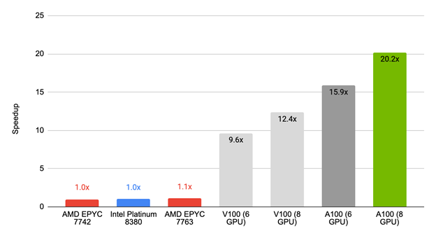
Figure 2. Simcenter STAR-CCM+ 2022.1 performance for model LeMans 104M on GPUs in comparison to CPU-only execution shows the top performing platform, with 20x higher speed, is the NVIDIA A100 PCIe 80GB.
Figure 2 shows the performance of the first release of Simcenter STAR-CCM+ 2022.1 against commonly available CPU-only servers. For the tested benchmark, an NVIDIA GPU-equipped server delivers results almost 20x faster than over 100 cores of CPU.
The AMD EPYC 7763 achieved 10% speedup of 1.1x, compared to the NVIDIA V100 (six GPUs) with a 9.6x speedup, NVIDIA V100 (eight GPUs) with a 12.4x speedup, NVIDIA A100 (six GPUs) with a 15.9x speedup, and NVIDIA A100 (eight GPUs) with a 20.2x speedup.
To put that into more practical terms, this means a simulation that takes a full day on a CPU server could be done in a little over an hour with a single node and eight NVIDIA A100 GPUs.
With the Simcenter STAR-CCM+ team continuing to work on improving and optimizing their GPU offering, you can expect even better performance in upcoming releases.
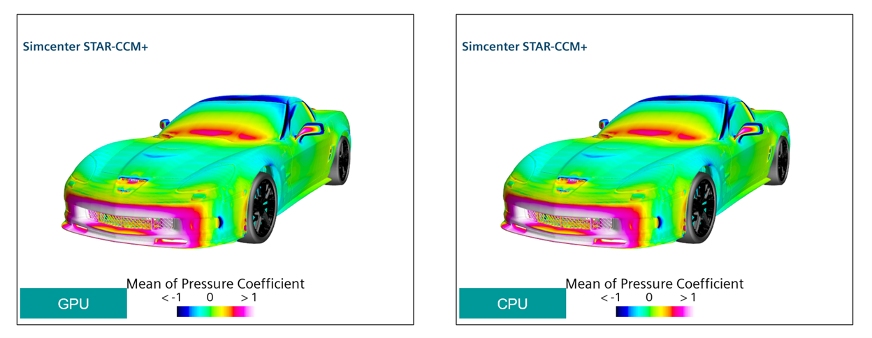
Figure 3. Simcenter STAR-CCM+ results for the mean of pressure coefficient compared between (left)GPU- and (right)CPU-based runs.
Corvette C6 ZR1 external aerodynamics, pseudo-steady simulation, 110M cells run with SST-DDES and Moving Reference Frame (MRF) for the wheels. GPU runs on 4xA100 DGX station.
GPU-accelerated runs are delivering consistent results compared to CPU-only runs, and Siemens delivered a product that can be seamlessly moved from CPUs to GPUs to get the results faster and effortlessly. The result is that you can now run simulations on-premises or on the cloud, as A100 GPU instances are available from all the major cloud service providers.
Siemens showed similar results in their announcement of GPU support in version 2022.1 when comparing CPU-only servers on-premises and in the cloud for both previous-generation V100 GPUs and current generation A100 GPUs. They also showed the performance of a large, industrial-scale model and the equivalent number of CPU cores required to get similar run times as that of a single node with eight GPUs on it.
Never to be left behind on technology trends, NVIDIA and Ansys announced the public beta availability of a GPU-accelerated, limited-functionality Fluent at the 2021 GTC Fall keynote.
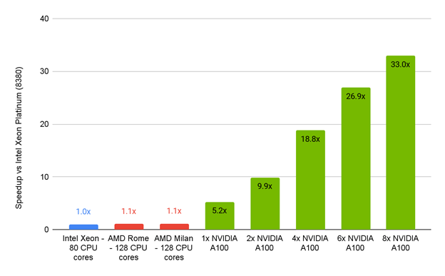
Figure 4. Performance of Ansys FLUENT 2022 beta1 for a 105M cell car model server vs. CPU-only servers.
This comparison is based on a 100-iteration timing, steady-state, GEKO turbulence model.
The performance of the Ansys Fluent 2022 beta1 server compared to CPU-only servers shows that Intel Xeon, AMD Rome, and AMD Milan had ~1.1x speedups compared to the NVIDIA A100 PCIe 80GB, which had speedups from 5.2x (one GPU) to an impressive 33x (eight GPUs).
The Ansys Fluent numbers drove some major excitement. They showed that a single GPU accelerated server for their selected benchmark and associated physics could deliver nearly 33x the performance of the standard Intel processor-only servers common today.
Such fast turnaround times are due to GPU acceleration of the two most used commercial CFD applications. This means that design engineers can not only incorporate simulations earlier into their design cycles but also explore several design iterations within a single day. They can make informed decisions about product performance quickly instead of having to wait for weeks.
Other options for GPU acceleration
At such speeds, other bottlenecks in the product research process can emerge. Sometimes a major consumer of engineering time is preprocessing, or the manual process of building the models to be run.
It is especially important to address this problem because it takes engineering person-time to solve. This is different from other factors, like simulation run time, that leave the researcher free to concentrate on other tasks. This is an active area of focus recently highlighted in CFD Mesh Generators: Top 3 Reasons They Slow Analysis and How to Fix Them.
All that said though, GPU acceleration is not an entirely new phenomenon. Some of the more niche tools have either been born in a GPU-accelerated world or have come to it sooner rather than later:
Altair CFD (NanoFluidX and UltraFluidX)
Cascade Technologies, CharLES
ESS Rocky
CPFD Barracuda
Dassault, XFlow
M-STAR CFD
NASA, FUN3D
NVIDIA has featured exciting and visually stunning results from NASA’s FUN3D tool, including the time Jensen Huang shared a simulation of a Mars lander entering the atmosphere.
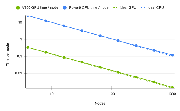
Figure 5. A 72-84x improvement shown for CPU vs. GPU performance of FUN3D version 14.0 (unreleased), courtesy of the NASA FUN3D team.
Hardware access provided by ORNL Summit using IBM AC922 Dual Power9 CPUs with 6x NVIDIA V100 SXM2 16 GB 2x EDR InfiniBand.
The most recent Supercomputing Conference featured research by a team that studied algorithmic changes which produce reductions in floating-point atomic updates required by large-scale parallel GPU computing environments. The runtime of several kernels is dominated by the update speeds, and therefore efficiencies found in this area have the potential for large benefits. Also, though FUN3D is a NASA and United States government-only tool, the discussion in this paper has applicability to other unstructured Reynolds-averaged Navier-Stokes CFD tools.
Beyond savings and removing roadblocks, maybe the most exciting part of mainstream CFD tools becoming GPU-accelerated is the new science and engineering that cut runtimes by factors of 15–30x. Until now, without access to leadership-class supercomputing capabilities, investigations into these areas have been too difficult from both a runtime and a problem-size standpoint:
Vehicle underhood modeling: Turbulent flow with heat transfer
Large eddy and combustion: Needed for detailed environmental emissions modeling
Magneto-hydrodynamics: Flows influenced by magnetic fields important to modeling fusion energy generators, internals of stars and gas giant planets
Machine learning training: Automatic generation of models and solutions that are used to train machine learning algorithms to estimate flow initial conditions, model turbulence, mixing, and so on
For more information about accelerated computing being used for other fluids or industrial simulations, watch the recommended recent GTC 2022 sessions focused on manufacturing and HPC:
It’s a beautiful day to play video games. And it’s GFN Thursday, which means we’ve got those games. Ten total titles join the GeForce NOW library of over 1,300 games, starting with the release of Roller Champions – a speedy, free-to-play roller skating title launching with competitive season 0. Rollin’ Into the Weekend Roll with Read article >
Can machines experience emotions? They might, according to Hume AI, an AI research lab and technology company that aims to “ensure artificial intelligence is built to serve human goals and emotional well-being.” So how can AI genuinely understand how we are feeling, and respond appropriately? On this episode of NVIDIA’s AI Podcast, host Noah Kravitz Read article >
Recalling the French linguist who deciphered the Rosetta Stone 150 years ago, Hewlett Packard Enterprise today switched on a tool to unravel its customers’ knottiest problems. The Champollion AI supercomputer takes its name from Jean-François Champollion (1790-1832), who decoded hieroglyphics that opened a door to study of ancient Egypt’s culture. Like Champollion, the mega-system resides Read article >
We built BenchBot to allow roboticists to spend more time researching the exciting and interesting problems in robotics. This post tells BenchBot’s story.
Working on robotics is full of exciting and interesting problems but also days lost to humbling problems like sensor calibration, building transform trees, managing distributed systems, and debugging bizarre failures in brittle systems.
We also recently upgraded to the new NVIDIA Omniverse-powered NVIDIA Isaac Sim, which has bought a raft of significant improvements to the BenchBot platform. Whether robotics is your hobby, academic pursuit, or job, BenchBot along with NVIDIA Isaac Sim capabilities enables you to jump into the wonderful world of robotics with only a few lines of Python. In this post, we share how we created BenchBot, what it enables, where we plan to take it in the future, and where you can take it in your own work. Our goal is to give you the tools to start working on your own robotics projects and research by presenting ideas about what you can do with BenchBot. We also share what we learned when integrating with the new NVIDIA Isaac Sim.
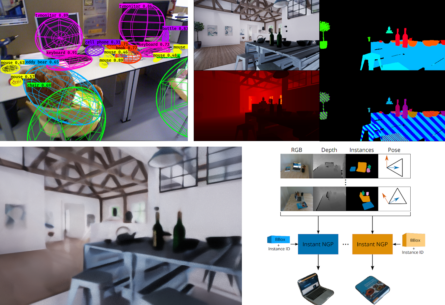
Figure 1. BenchBot gives users access to 25 photorealistic environments out of the box, with variations in lighting and objects present (see the BEAR dataset)
This post also supplies context for our Robotic Vision Scene Understanding (RVSU) challenge, currently in its third iteration. The RVSU challenge is a chance to get hands-on in trying to solve a fundamental problem for domestic robots: how can they understand what is in their environment, and where. By competing, you can win a share in prizes including NVIDIA A6000 GPUs and $2,500 USD cash.
The story behind BenchBot
BenchBot addressed a need in our semantic scene understanding research. We’d hosted an object detection challenge and produced novel evaluation metrics but needed to expand this work to the robotics domain:
What is understanding a scene?
How can the level of understanding be evaluated?
What role does agency play in understanding a scene?
Can understanding in simulation transfer to the real world?
What’s required of a simulation for understanding to transfer to the real world?
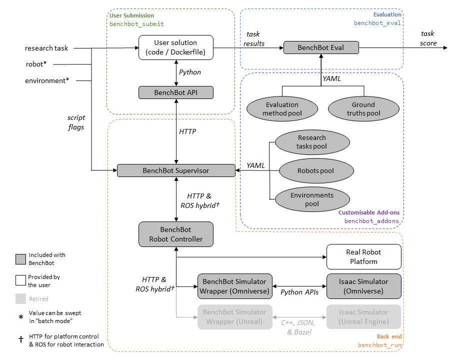
We made the BenchBot platform to enable you to focus on these big questions, without becoming lost in the sea of challenges typically thrown up by robotic systems. BenchBot consists of many moving parts that abstract these operational complexities away (Figure 2).
Figure 2. System overview of the BenchBot platform
Here are some of the key components and features of the BenchBot architecture:
You create solutions to robotics problems by writing a Python script that calls the BenchBot API.
You can easily understand how well your solution performed a given robotics task using customisable evaluation tools.
The supervisor brokers communications between the high-level Python API and low-level interfaces of typical robotic systems.
The supervisor is backend-agnostic. The robot can be real or simulated, it just needs to be running ROS.
All configurations live in a modular add-on system, allowing you to easily extend the system with your own tasks, robots, environments, evaluation methods, examples, and more.
A lot of moving parts isn’t necessarily a good thing if they complicate the user experience, so designing the user experience was also a central focus in developing BenchBot.
There are three basic commands for controlling the system:
With a simple Python API, world-class photorealistic simulation, and only a handful of commands needed to manage the entire system, we were ready to apply BenchBot to our first big output: the RVSU challenge.
RVSU challenge
The RVSU challenge prompts researchers to develop robotic vision systems that understand both the semantic and geometric aspects of the surrounding environment. The challenge consists of six tasks, featuring multiple difficulty levels for object-based, semantic, simultaneous localization and mapping (SLAM) and scene change detection (SCD).
The challenge also focuses on a core requirement for household robots: they need to understand what objects are in their environment, and where they are. This problem in itself is the first challenge captured in our semantic SLAM tasks, where a robot must explore an environment, find all objects of interest, and add them to a 3D map.
The SCD task takes this a step further, asking a robot to report changes to the objects in the environment at a different point in time. My colleague David Hall presented an excellent overview of the challenge in the following video.
Video 1. Scene Understanding Challenges
Bringing the RVSU challenge to life with NVIDIA Isaac Sim
Recently, we upgraded BenchBot from using the old Unreal Engine-based NVIDIA Isaac Sim to the new Omniverse-powered NVIDIA Isaac Sim. This brought a number of key benefits to BenchBot, leaving us excited about where we can go with Omniverse-powered simulations in the future. The areas in which we saw significant benefits included the following:
Quality: NVIDIA RTX rendering produced beautiful photorealistic simulations, all with the same assets that we were using before.
Performance: We accessed powerful dynamic lighting effects, with intricately mapped reflections, all produced in real-time for live simulation with realistic physics.
Customizability: The Python APIs for Omniverse and NVIDIA Isaac Sim give complete control of the simulator, allowing us to restart simulations, swap out environments, and move robots programmatically.
The qcr/benchbot_sim_omni repository captures our learnings in transitioning to the new NVIDIA Isaac Sim, and also works as a standalone package outside the BenchBot ecosystem. The package is a customizable HTTP API for loading environments, placing robots, and controlling simulations. It serves as a great starting point for programmatically running simulations with NVIDIA Isaac Sim.
We welcome pull requests and suggestions for how to expand the capabilities of this package. We also hope it can offer some useful examples for starting your own projects with NVIDIA Isaac Sim, such as the following examples.
Opening environments in NVIDIA Isaac Sim
Opening environments first requires a running simulator instance. A new instance is created by instantiating the SimulationApp class, with the open_usd option letting you pick an environment to open initially:
It’s worth noting that only one simulation instance can run per Python script, and NVIDIA Isaac Sim components must be imported after initializing the instance.
Select a different stage at runtime by using helpers in the NVIDIA Isaac Sim API:
python
from omni.isaac.core.utils.stage import open_stage, update_stage

open_stage(usd_path=MAP_USD_PATH)
update_stage()
Placing a robot in the environment
Before starting a simulation, load and place a robot in the environment. Do this with the Robot class and the following lines of code:
Simulations in NVIDIA Isaac Sim are controlled by the SimulationContext class:
python
from omni.isaac.core import SimulationContext
sim = SimulationContext()
sim.play()
Then, the step method gives fine-grained control over the simulation, which runs at 60Hz. We used this control to manage our sensor publishing, transform trees, and state detection logic.
Another useful code example we stumbled upon was using the dynamic_control module to get the robot’s ground truth pose during a simulation:
python
from omni.isaac.dynamic_control import _dynamic_control
dc = _dynamic_control.acquire_dynamic_control_interface()
robot_dc = dc.get_articulation_root_body(dc.get_object(ROBOT_PRIM_PATH))
gt_pose = dc.get_rigid_body_pose(robot_dc)
Results
Hopefully these code examples are helpful to you in getting started with NVIDIA Isaac Sim. With not much more than these, we’ve had some impressive results:
A remarkable improvement in our photorealistic simulations
Powerful real-time lighting effects
Full customization through basic Python code
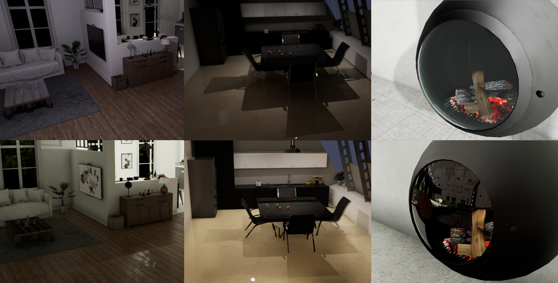
Figures 3, 4, and 5 show some of our favorite visual improvements from making the transition to Omniverse.
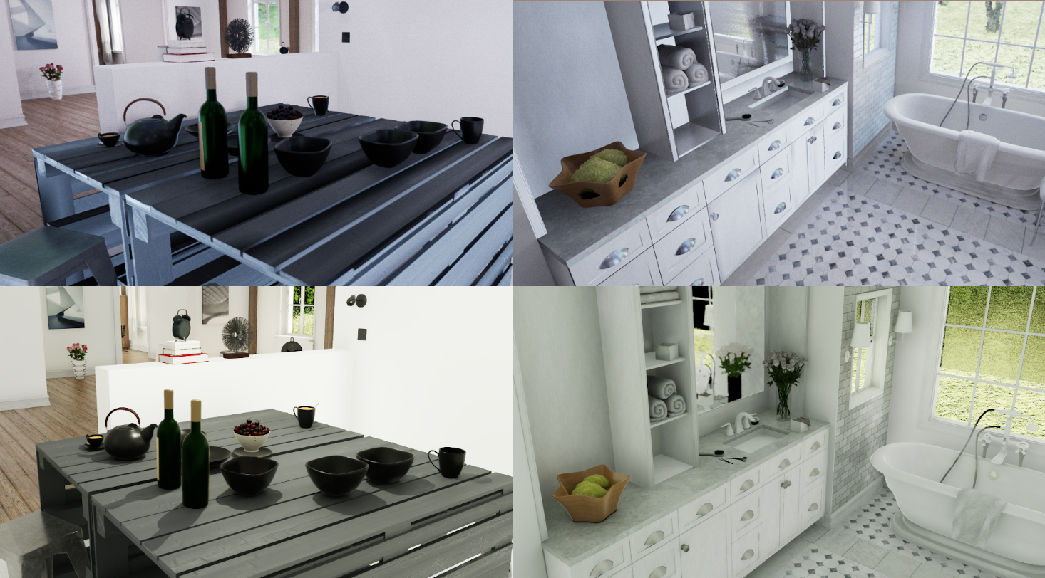
Figure 3. Surfaces give more realistic reflections in the new NVIDIA Isaac Sim (bottom row) than the previous version (top row)
Figure 4. Shadows and texture rendering feels more realistic in the new NVIDIA Isaac Sim (bottom row) than they previously did (top row)
Figure 5. New NVIDIA Isaac Sim leads to environments that feel more immersive (right), with previous environments (left) feeling “flat” in comparison
Taking it further: BenchBot in other domains
Although semantic scene understanding is a focal point of our research and the origins of its use in research, BenchBot’s applications aren’t limited solely to this domain. BenchBot is built using a rich add-on architecture allowing modular additions and adaptations of the system to different problem domains.
The visual learning and understanding research program at QCR has started using this flexibility to apply BenchBot and its Omniverse-powered simulations to a range of interesting problems. Figure 6 shows a few areas where we’re looking at employing BenchBot:
Figure 6. Future uses for BenchBot, clockwise from top-right: semantic mapping with quadrics, synthetic datasets with object-level segmentation, object-level NeRFs from noisy data, and understanding scenes with NeRFs
We’ve made BenchBot with a heavy focus on being able to fit it to your research problems. As much as we’re enjoying applying it to our research problems, we’re excited to see where others take it. Creating your own add-ons is documented in the add-ons repository, and we’d love to add some third-party add-ons to the official add-ons organization.
Conclusion
We hope this in-depth review has been insightful, and helps you step into robotics to work on the problems that excite us roboticists.
We welcome entries for the RVSU challenge, whether your interest in semantic scene understanding is casual or formal, academic or industrial, competitive or iterative. We think you’ll find competing in the challenge with the BenchBot system an enriching experience. You can register for the challenge, and submit entries through the EvalAI challenge page.
If you’re looking for where to go next with BenchBot and Omniverse, here are some suggestions:
Contact BenchBot’s authors if you’ve got ideas for research collaboration or problems where you’d like to apply it.
At QCR, we’re excited to see where robotics is heading. With tools like BenchBot and the new Omniverse-powered NVIDIA Isaac Sim, there’s never been a better time to jump in and start playing with robotics.
filenames = glob.glob(str(pathlib.Path('/content/maestro-v2.0.0/')/'**/*.mid*')) all_notes = [] for f in filenames[:5]: notes = midi_to_df(f) all_notes.append(notes) notes_df = pd.concat(all_notes) key_order = ['pitch', 'step', 'duration'] train_notes = np.stack([all_notes[key] for key in key_order], axis=1) notes_ds = tf.data.Dataset.from_tensor_slices(train_notes) notes_ds.element_spec
Then get this error:
Traceback (most recent call last) <ipython-input-70-eeb27cd23560> in <module>() 13 notes_df = pd.concat(all_notes) 14 key_order = ['pitch', 'step', 'duration'] ---> 15 train_notes = np.array([all_notes[key] for key in key_order], axis=1) 16 notes_ds = tf.data.Dataset.from_tensor_slices(train_notes) 17 notes_ds.element_spec <ipython-input-70-eeb27cd23560> in <listcomp>(.0) 13 notes_df = pd.concat(all_notes) 14 key_order = ['pitch', 'step', 'duration'] ---> 15 train_notes = np.array([all_notes[key] for key in key_order], axis=1) 16 notes_ds = tf.data.Dataset.from_tensor_slices(train_notes) 17 notes_ds.element_spec TypeError: list indices must be integers or slices, not str
Any help would be appreciated. I’ve spent the last two weeks going through every tutorial I can find and it feels like literally not a single one works without an error every five lines that takes me two hours to research how to fix, some are easy, but all of them lead to something I can’t figure out, and I give up. I am determined to get one of these to work. And this one seems to simple but ofc I’ve reached a point I can’t figure out. PLEASE help me out here. thank you
Autonomous parking involves complex perception algorithms. We present an AI-based parking sign assist system relying on live perception that can fuse to map systems.
Here’s the latest video in the NVIDIA DRIVE Labs series. These videos take an engineering-focused look at individual autonomous vehicle challenges and how the NVIDIA DRIVE team is mastering them. Catch up on more NVIDIA DRIVE posts.
Autonomous parking involves an array of complex perception and decision-making algorithms and traditionally relies on high-definition (HD) maps to retrieve parking information.
However, map coverage and poor or outdated localization information can limit such systems. Adding to this complexity, the system must understand and interpret parking rules that vary from region to region.
In this DRIVE Labs post, we show how AI-based live perception can help scale autonomous parking to regions across the globe.
Video 1. Advancing Autonomous Valet Functionality with Parking Sign Assist
Autonomous parking system overview
Understanding and interpreting parking rules can be more nuanced than it appears.
Different parking rules within the effective region can be overridden. For example, “No Stopping” can overwrite “No Parking.”
In addition, nonparking-related signs can infer parking rules. For example, in Germany, parking is not allowed within 15 meters of any bus stop signs. In the U.S., parking is illegal within 30 feet before a stop sign.
Finally, besides explicit clues like a physical sign, there are implicit signs that carry parking information. For example, in many areas, an intersection indicates the end of the previous active parking rule.
An advanced algorithm-based parking sign assist (PSA) system is critical for autonomous vehicles to understand the complexity of parking rules and react accordingly.
Traditional PSA systems rely on input from HD maps alone. However, the NVIDIA DRIVE AV software stack leverages state-of-the-art deep neural networks (DNNs) and computer vision algorithms to improve the coverage and robustness of autonomous parking in real-world scenarios. These techniques can detect, track, and classify a wide variety of parking traffic signs and road intersections in real time.
The WaitNet DNN detects traffic signs and intersections.
The wait perception stack tracks individual signs and intersections to provide 3D positions through triangulation.
The results from the modules are then fed into the PSA system, which uses the data to determine whether the car is in a parking strip, what the restrictions are, and whether the car is allowed to stop or park within the region.
Parking sign assist overview
After the PSA system receives the detected parking signs and road intersections, it abstracts the object into a Start Parking Sign or an End Parking Sign. This level of abstraction allows the system to scale worldwide.
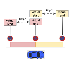
A Start Parking Sign marks a potential start of a new parking strip and an End Parking Sign may close one or more existing parking strips. Figures 1 and 2 show how parking strips are formed.
Figure 1. Forming parking strips
Figure 1 abstracts signs and road intersections to form parking strips. The diagram shows that a single sign can generate multiple virtual signs. For example, the sign in the middle serves as the “end” sign for the leftmost sign and it serves as the “start” for the rightmost sign.
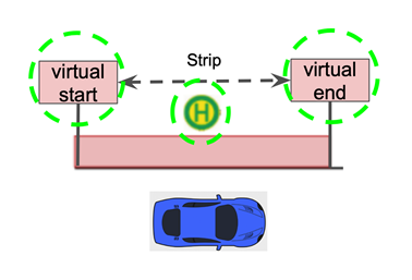
Figure 2. A car alongside a no parking zone.
In addition to forming a parking strip, the PSA system uses the semantic meaning of signs to classify a parking strip as no-parking, no-stopping, parking-allowed, and unknown states. Then this information can be provided to the driver or any autonomous parking system.
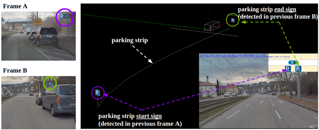
Figure 3. The high-level working of a PSA
Figure 3 shows the main function workflow of the PSA system. In Frame A, the “Parking Area Start” sign is detected and a new parking strip is created. After the car drives a while, a “Parking Area End” sign is detected, which matches the start sign of that parking strip.
Finally, the PSA system stores all active parking strips in its memory and signals the driver the current parking status based on traffic rules implied by the parking strip in effect.
Conclusion
The PSA system achieves complex decision-making with remarkable accuracy, running in just a few milliseconds on NVIDIA DRIVE AGX. It is also compatible with any perception-only autonomous vehicle stack that uses live camera sensor input.
Our current SignNet DNN supports more than 20 parking signs in Europe, including bus stop signs, no parking signs, and no stopping signs, with coverage continuing to expand. We are also adding optical character recognition (OCR) and natural language processing (NLP) modules into the system to handle complex information carried by written texts on the signs.
To learn more about the software functionality that we are building, see the rest of the NVIDIA DRIVE Lab video series.
NVIDIA today reported record revenue for the first quarter ended May 1, 2022, of $8.29 billion, up 46% from a year ago and up 8% from the previous quarter, with record revenue in Data Center and Gaming…
Posted by Pasin Manurangsi and Chiyuan Zhang, Research Scientists, Google Research
Over the last several years, there has been an increased focus on developing differential privacy (DP) machine learning (ML) algorithms. DP has been the basis of several practical deployments in industry — and has even been employed by the U.S. Census — because it enables the understanding of system and algorithm privacy guarantees. The underlying assumption of DP is that changing a single user’s contribution to an algorithm should not significantly change its output distribution.
In the standard supervised learning setting, a model is trained to make a prediction of the label for each input given a training set of example pairs {[input1,label1], …, [inputn, labeln]}. In the case of deep learning, previous work introduced a DP training framework, DP-SGD, that was integrated into TensorFlow and PyTorch. DP-SGD protects the privacy of each example pair [input, label] by adding noise to the stochastic gradient descent (SGD) training algorithm. Yet despite extensive efforts, in most cases, the accuracy of models trained with DP-SGD remains significantly lower than that of non-private models.
DP algorithms include a privacy budget, ε, which quantifies the worst-case privacy loss for each user. Specifically, ε reflects how much the probability of any particular output of a DP algorithm can change if one replaces any example of the training set with an arbitrarily different one. So, a smaller ε corresponds to better privacy, as the algorithm is more indifferent to changes of a single example. However, since smaller ε tends to hurt model utility more, it is not uncommon to consider ε up to 8 in deep learning applications. Notably, for the widely used multiclass image classification dataset, CIFAR-10, the highest reported accuracy (without pre-training) for DP models with ε = 3 is 69.3%, a result that relies on handcrafted visual features. In contrast, non-private scenarios (ε = ∞) with learned features have shown to achieve >95% accuracy while using modern neural network architectures. This performance gap remains a roadblock for many real-world applications to adopt DP. Moreover, despite recentadvances, DP-SGD often comes with increased computation and memory overhead due to slower convergence and the need to compute the norm of the per-example gradient.
In “Deep Learning with Label Differential Privacy”, presented at NeurIPS 2021, we consider a more relaxed, but important, special case called label differential privacy (LabelDP), where we assume the inputs (input1, …, inputn) are public, and only the privacy of the training labels (label1, …, labeln) needs to be protected. With this relaxed guarantee, we can design novel algorithms that utilize a prior understanding of the labels to improve the model utility. We demonstrate that LabelDP achieves 20% higher accuracy than DP-SGD on the CIFAR-10 dataset. Our results across multiple tasks confirm that LabelDP could significantly narrow the performance gap between private models and their non-private counterparts, mitigating the challenges in real world applications. We also present a multi-stage algorithm for training deep neural networks with LabelDP. Finally, we are excited to release the code for this multi-stage training algorithm.
LabelDP The notion of LabelDP has been studied in the Probably Approximately Correct (PAC) learning setting, and captures several practical scenarios. Examples include: (i) computational advertising, where impressions are known to the advertiser and thus considered non-sensitive, but conversions reveal user interest and are thus private; (ii) recommendation systems, where the choices are known to a streaming service provider, but the user ratings are considered sensitive; and (iii) user surveys and analytics, where demographic information (e.g., age, gender) is non-sensitive, but income is sensitive.
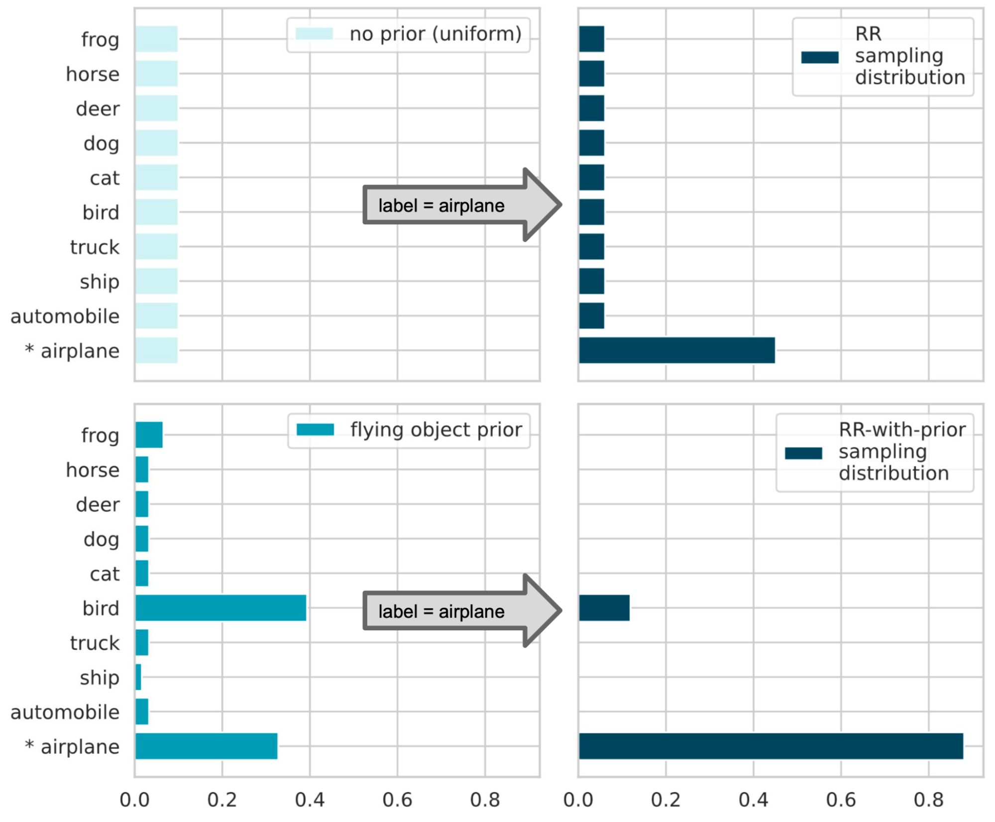
We make several key observations in this scenario. (i) When only the labels need to be protected, much simpler algorithms can be applied for data preprocessing to achieve LabelDP without any modifications to the existing deep learning training pipeline. For example, the classic Randomized Response (RR) algorithm, designed to eliminate evasive answer biases in survey aggregation, achieves LabelDP by simply flipping the label to a random one with a probability that depends on ε. (ii) Conditioned on the (public) input, we can compute a prior probability distribution, which provides a prior belief of the likelihood of the class labels for the given input. With a novel variant of RR, RR-with-prior, we can incorporate prior information to reduce the label noise while maintaining the same privacy guarantee as classical RR.
The figure below illustrates how RR-with-prior works. Assume a model is built to classify an input image into 10 categories. Consider a training example with the label “airplane”. To guarantee LabelDP, classical RR returns a random label sampled according to a given distribution (see the top-right panel of the figure below). The smaller the targeted privacy budget ε is, the larger the probability of sampling an incorrect label has to be. Now assume we have a prior probability showing that the given input is “likely an object that flies” (lower left panel). With the prior, RR-with-prior will discard all labels with small prior and only sample from the remaining labels. By dropping these unlikely labels, the probability of returning the correct label is significantly increased, while maintaining the same privacy budget ε (lower right panel).
Randomized response: If no prior information is given (top-left), all classes are sampled with equal probability. The probability of sampling the true class (P[airplane] ≈ 0.5) is higher if the privacy budget is higher (top-right). RR-with-prior: Assuming a prior distribution (bottom-left), unlikely classes are “suppressed” from the sampling distribution (bottom-right). So the probability of sampling the true class (P[airplane] ≈ 0.9) is increased under the same privacy budget.
A Multi-stage Training Algorithm Based on the RR-with-prior observations, we present a multi-stage algorithm for training deep neural networks with LabelDP. First, the training set is randomly partitioned into multiple subsets. An initial model is then trained on the first subset using classical RR. Finally, the algorithm divides the data into multiple parts, and at each stage, a single part is used to train the model. The labels are produced using RR-with-prior, and the priors are based on the prediction of the model trained so far.
An illustration of the multi-stage training algorithm. The training set is partitioned into t disjoint subsets. An initial model is trained on the first subset using classical RR. Then the trained model is used to provide prior predictions in the RR-with-prior step and in the training of the later stages.
Results We benchmark the multi-stage training algorithm’s empirical performance on multiple datasets, domains, and architectures. On the CIFAR-10 multi-class classification task for the same privacy budget ε, the multi-stage training algorithm (blue in the figure below) guaranteeing LabelDP achieves 20% higher accuracy than DP-SGD. We emphasize that LabelDP protects only the labels while DP-SGD protects both the inputs and labels, so this is not a strictly fair comparison. Nonetheless, this result demonstrates that for specific application scenarios where only the labels need to be protected, LabelDP could lead to significant improvements in the model utility while narrowing the performance gap between private models and public baselines.
Comparison of the model utility (test accuracy) of different algorithms under different privacy budgets.
In some domains, prior knowledge is naturally available or can be built using publicly available data only. For example, many machine learning systems have historical models which could be evaluated on new data to provide label priors. In domains where unsupervised or self-supervised learning algorithms work well, priors could also be built from models pre-trained on unlabeled (therefore public with respect to LabelDP) data. Specifically, we demonstrate two self-supervised learning algorithms in our CIFAR-10 evaluation (orange and green traces in the figure above). We use self-supervised learning models to compute representations for the training examples and run k-means clustering on the representations. Then, we spend a small amount of privacy budget (ε ≤ 0.05) to query a histogram of the label distribution of each cluster and use that as the label prior for the points in each cluster. This prior significantly boosts the model utility in the low privacy budget regime (ε < 1).
Similar observations hold across multiple datasets such as MNIST, Fashion-MNIST and non-vision domains, such as the MovieLens-1M movie rating task. Please see our paper for the full report on the empirical results.
The empirical results suggest that protecting the privacy of the labels can be significantly easier than protecting the privacy of both the inputs and labels. This can also be mathematically proven under specific settings. In particular, we can show that for convex stochastic optimization, the sample complexity of algorithms privatizing the labels is much smaller than that of algorithms privatizing both labels and inputs. In other words, to achieve the same level of model utility under the same privacy budget, LabelDP requires fewer training examples.
Conclusion We demonstrated that both empirical and theoretical results suggest that LabelDP is a promising relaxation of the full DP guarantee. In applications where the privacy of the inputs does not need to be protected, LabelDP could reduce the performance gap between a private model and the non-private baseline. For future work, we plan to design better LabelDP algorithms for other tasks beyond multi-class classification. We hope that the release of the multi-stage training algorithm code provides researchers with a useful resource for DP research.
Acknowledgements This work was carried out in collaboration with Badih Ghazi, Noah Golowich, and Ravi Kumar. We also thank Sami Torbey for valuable feedback on our work.


 The end of 2021 and beginning of 2022 saw the two largest commercial CFD tool vendors, Ansys and Siemens, both launch versions of their flagship CFD tools with support for GPU acceleration.
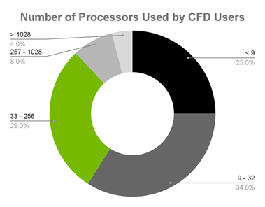
") We built BenchBot to allow roboticists to spend more time researching the exciting and interesting problems in robotics. This post tells BenchBot’s story.
We built BenchBot to allow roboticists to spend more time researching the exciting and interesting problems in robotics. This post tells BenchBot’s story.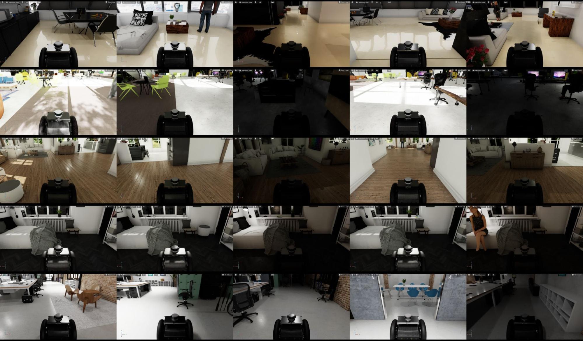

 Autonomous parking involves complex perception algorithms. We present an AI-based parking sign assist system relying on live perception that can fuse to map systems.