Categories
Misc

Training a State-of-the-Art ImageNet-1K Visual Transformer Model using NVIDIA DGX SuperPOD

This post shows how the SOTA Visual Transformer model, VOLO, is trained on the NVIDIA DGX SuperPOD. VOLO_D5 model.

Recent work has demonstrated that large transformer models can achieve or advance the SOTA in computer vision tasks such as semantic segmentation and object detection. However, unlike convolutional network models that can do it only with the standard public dataset, it takes a proprietary dataset that is magnitudes larger.

VOLO model architecture

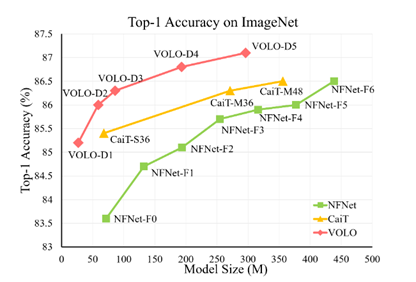
The recent project VOLO (Vision Outlooker) from SEA AI Lab, Singapore showed an efficient and scalable vision transformer mode architecture that greatly closed the gap using only the ImageNet-1K dataset.

VOLO introduces a novel outlook attention and presents a simple and general architecture, termed Vision Outlooker. Unlike self-attention, which focuses on global dependency modeling at a coarse level, the outlook attention efficiently encodes finer-level features and contexts into tokens. This is shown to be critically beneficial to recognition performance but largely ignored by self-attention.

Experiments show that the VOLO achieves 87.1% top-1 accuracy on ImageNet-1K classification, which is the first model exceeding 87% accuracy on this competitive benchmark, without using any extra training data.

Chart shows that the VOLO model has outperformed the state of the art image recognition models at different model complexity levels respectively in terms of Top-1 accuracy. For example, VOLO-D5 achieved more than 87% Top-1 accuracy.
Figure 1. Top-1 Accuracy of VOLO models in different sizing levels

In addition, the pretrained VOLO transfers well to downstream tasks, such as semantic segmentation.

Settings LV-ViT  CaiT NFNet-F6 NFNNet-F5 VOLO-D5
Test Resolution 448×448 448×448 576×576 544×544 448×448/512×512
Model Size 140M 356M 438M 377M 296M
Computations 157B 330B 377B 290B 304B/412B
Architecture Vision Transformer Vision Transformer Convolutions Convolutions VOLO
Extra Augmentations Token Labeling Knowledge Distill SAM SAM+augmult Token Labeling
ImageNet Top-1 Acc. 86.4 86.5 86.5 86.8 87.0/87.1
Table 1. Overview of the compared ViT, CNN baseline models

Though VOLO models demonstrated outstanding computational efficiency, training the SOTA performance model is not trivial. 

In this post, we present the techniques and experience that we gained training the VOLO models on the NVIDIA DGX SuperPOD based on the NVIDIA ML software stack and Infiniband clustering technologies.

Training methods

Training VOLO models requires considering training strategy, infrastructure, and configuration planning.  In this section, we discuss some of the techniques applied in this solution.

Training strategy

Training the model using the original ImageNet sample quality data all the way and performing a neural network (NN) architecture search at a fine grain makes a more consolidated investigation in theory. However, this requires a large percentage of the computing resources budget.

In the scope of this project, we adopted a coarse-grained training approach that does not visit as many NN architecture possibilities as the fine-grained approach. However, it enables showing EIOFS with less time and a lower resource budget. In this alternative strategy, we first trained the potential neural network candidates using image samples with lower resolution and then performed fine-tuning using high-resolution images.

This approach has been proved to be efficient in earlier work in terms of cutting down the computational cost within marginal model performance lost.

Infrastructure

In practice, we used two types of clusters for this training:

  • One for base model pretraining, which is an NVIDIA DGX A100 based DGX POD that consists of 5x NVIDIA DGX A100 systems clustered using the NVIDIA Mellanox HDR Infiniband network.
  • One for fine-tuning, which is an NVIDIA DGX SuperPOD that consists of DGX A100 systems with the NVIDIA Mellanox HDR Infiniband network. 
Diagram shows the DGX POD/SuperPOD hardware and infiniband network, on the compute front, APEX for enabling scalable mixed precision compute and on the networking front, NVIDIA PyXis and NCCL are leveraged for best using the DGX A100 GPU networking capability.
Figure 2. NVIDIA technology-based software stack used in this project

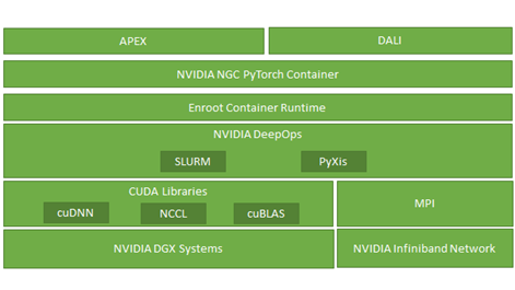
Software infrastructure also played important role in this procedure. Figure 2 shows that, in addition to the underlying standard deep learning optimization CUDA  libraries such as cuDNN and cuBLAS, we leveraged NCCL, enroot, PyXis, APEX, and DALI  extensively to achieve the sub-linear scalability of the training performance.

The DGX A100 POD cluster is mainly used for base model pretraining using lower size image samples. This is because base model pretraining is less memory-bound and can leverage the compute power advantage of the NVIDIA A100 GPU.

In comparison, the fine-tuning was performed on an NVIDIA DGX SuperPOD of NVIDIA DGX-2 because the fine-tuning process uses bigger images, which requires more memory per compute power. 

Training configurations

NEED LEAD-IN SENTENCE

  D1 D2 D3 D4 D5
MLP Ratio 3 3 3 3 4
Optimizer AdamW
LR Scaling LR = LRbase x Batch_Size/1024,    where LRbase=8.0e-4
Weight Decay 5e-2
LRbase 1.6e-2 1e-3 1e-3 1e-3 1e-4
Stochastic Depth Rate 0.1 0.2 0.5 0.5 0.75
Crop Ratio 0.96 0.96 0.96 1.15 1.15

Table 2. Model settings (for all models, the batch size is set to 1024)

We evaluated our proposed VOLO models on the ImageNet dataset. During training, no extra training data was used. Our code was based on PyTorch, the Token Labeling toolbox, and PyTorch Image Models (timm). We used the LV-ViT-S model with Token Labeling as our baseline.

Setup notes

  • We used the AdamW optimizer with a linear learning rate scaling strategy LR = LRbase x Batch_Size/1024 and 5 ×10⁻² weight decay rate as suggested by previous work, and LRbase are given in Table 3 for all VOLO models.
  • Stochastic Depth is used.
  • We trained our models on the ImageNet dataset for 300 epochs.
  • For data augmentation methods, we used CutOut, RandAug, and the Token Labeling objective with MixToken.
  • We did not use MixUp or CutMix as they conflict with MixToken.

Pretraining

In this section, we use VOLO-D5 as an example to demonstrate how the model is trained.

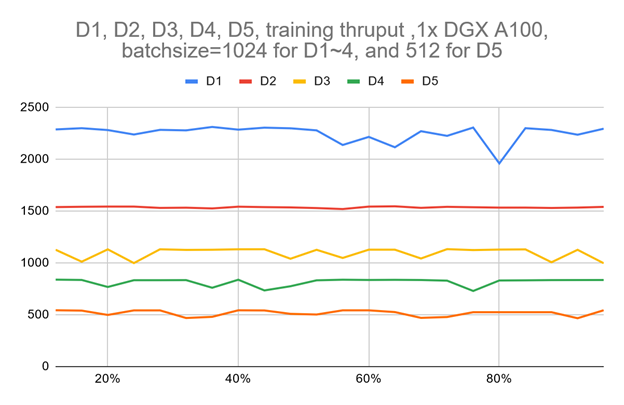
Figure 3 shows that the training throughput for VOLO-D5 using one single DGX A100 is about 500 image/sec. By estimation, it roughly takes about 170 hours to finish one full pretraining cycle, which needs 300 epochs with ImageNet-1K. This is equal to about one week for 1 million images.

To speed up a little bit, based on a simple parameter-server architecture cluster of five DGX A100 nodes, we roughly achieved a 2100 image/sec throughput, which can cut down the pretraining time to ~52 hours.

Chart shows that the training throughput of VOLO D1 to D5 models varies from 2300 img/sec to 500 img/sec on one single DGX A100 node when batch size is configured to 1024.
Figure 3. Training throughput of D1~D5 model on one single DGX A100 across one full epoch

The VOLO-D5 model pretraining can be started on one single node using the following code example:

CUDA_VISIBLE_DEVICES=0,1,2,3,4,5,6,7 ./distributed_train.sh 8 /path/to/imagenet 
  --model volo_d5 --img-size 224 
  -b 44 --lr 1.0e-4 --drop-path 0.75 --apex-amp 
  --token-label --token-label-size 14 --token-label-data /path/to/token_label_data

For the MNMG training case, it requires training cluster details as part of the command line input. First, we set CPU, MEM, IB Binding according to the node and cluster architecture. The cluster for the pre-training phase was DGX A100 POD, which has four NUMA domains per CPU socket and 1 IB port per A100 GPU, therefore we bind each rank to all CPU cores in the NUMA node nearest its GPU.

  • For memory binding, we bind each rank to the nearest NUMA node.
  • For IB binding, we bind one IB card per GPU, or as close to such a setup as possible.

Because the VOLO model training is PyTorch-based, and simply leveraged on the default PyTorch distributed training approach, our multinode, multi-GPU training is based on a simple parameter-server architecture that fits into the fat-tree network topology of NVIDIA DGX SuperPOD.

To simplify the scheduling, the first node in the list of allocated nodes is always used as both parameter server and worker node, and all other nodes are worker nodes. To avoid the potential storage I/O overhead, the dataset, all code, intermediate/milestone checkpoints, and results are kept on a single high-performance DDN-based distributed storage backend. They are mounted to all the worker nodes through a 100G NVIDIA Mellanox EDR Infiniband network.

To accelerate the data preprocessing and pipelining data loading, NVIDIA DALI is configured to use one dedicated data loader per GPU process. 

Diagram shows the training throughput speed up using two different generations of GPU, which are NVIDIA A100 and V100 GPUs  in the model pre-training phase. The workload scales out linearly on both GPUs but A100s apparently scales faster.
Figure 4. Pretraining phase training throughput speed up against the number of A100 and V100 GPUs

Fine-tuning

Running VOLO-D5 model fine-tuning on one single node is quite straightforward using the following code example:

CUDA_VISIBLE_DEVICES=0,1,2,3,4,5,6,7 ./distributed_train.sh 8 /path/to/imagenet 
  --model volo_d5 --img-size 512 
  -b 4 --lr 2.3e-5 --drop-path 0.5 --apex-amp --epochs 30 
  --weight-decay 1.0e-8 --warmup-epochs 5  --ground-truth 
  --token-label --token-label-size 24 --token-label-data /path/to/token_label_data 
  --finetune /path/to/pretrained_224_volo_d5/

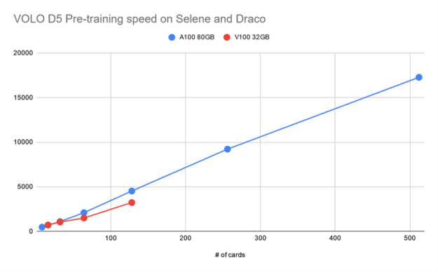
As we mentioned earlier, because the image size for fine-tuning is much larger than the one used in the pretraining phase, the batch size must be cut down accordingly. Get the workload to fit into the GPU memory, which makes further scaling out the training to larger numbers of GPUs in parallel mandatory.

Diagram shows the training throughput speed up using two different generations of GPU, which are NVIDIA A100 and V100 GPUs  in the model fine-tuning phase. DGX SuperPOD with DGX A100 provides significantly faster speed ramping up than the previous generation DGX SuperPOD.
Figure 5. Fine-tuning phase training throughput speed up against the number of A100 and V100 GPUs

Most of the fine-tuning configurations are similar to the pretraining phase.

Conclusion

In this post, we showed the main techniques and procedures for training the SOTA large-scale Visual Transformer models, such as VOLO_D5, on a large-scale AI supercomputer, such as NVIDIA DGX A100 based DGX SuperPOD. The trained VOLO_D5 model achieved the best Top-1 accuracy in the image classification model ranking without using any additional data beyond the ImageNet-1k dataset.

The code resource of this work including the Docker image for running the experiment and the Slurm scheduler script is open source in the sail-sg/volo GitHub repo to allow future work to be leveraged on VOLO_D5 for more extensive study. For more information, see VOLO: Vision Outlooker for Visual Recognition.

In the future, we are looking to scale this work further towards training more intelligent, self-supervised, larger-scale models with larger public datasets and more modern infrastructure, for example, NVIDIA DGX SuperPOD with NVIDIA H100 GPUs.

Categories
Misc

An Introduction to Edge Computing: Common Questions and Resources for Success

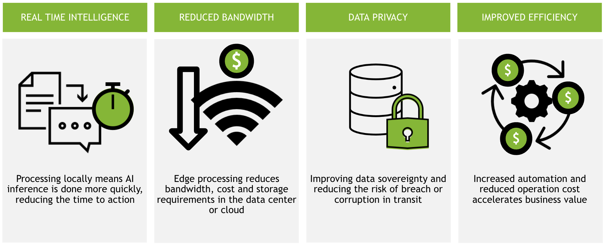
During a recent webinar, participants outlined common edge computing questions and challenges. This post provides NVIDIA resources to help beginners on their journey.

With the convergence of IoT and AI organizations are evaluating new ways of computing to keep up with larger data loads and more complicated use cases. For many, edge computing provides the right environment to successfully operate AI applications ingesting data from distributed IoT devices. 

But many organizations are still grappling with understanding edge computing. Partners and customers often ask about edge computing, reasons for its popularity in the AI space, and use cases compared to cloud computing. 

NVIDIA recently hosted an Edge Computing 101: An Introduction to the Edge webinar. The event provided an introduction to edge computing, outlined different types of edge, the benefits of edge computing, when to use it and why, and more. 

During the webinar, we surveyed the audience to understand their biggest questions about edge computing and how we could help. 

Below we provide answers to those questions, along with resources that could help you along your edge computing journey.  

What stage are you in, on your edge computing journey? 

About 51% of the audience answered that they are in the “learning” phase of their journey. At face value, this is not surprising given that the webinar was an introductory session. Of course most of the folks are at the learning phase, as opposed to implementing or scaling. This was also corroborated by the fact that many of the tools in the edge market are still new, meaning many vendors also have much to gain from learning more. 

To help in the learning journey refer to Considerations for Deploying AI at the Edge. This overview covers the major decision points for choosing the right components for an edge solution, security tips on edge deployments, and how to evaluate where edge computing fits into your existing environment. 

What is the top benefit you hope to gain by deploying applications at the edge? 

There are many benefits to deploying AI applications in edge computing environments, including real-time insights, reduced bandwidth, data privacy, and improved efficiency. For the participants in the session, 42% responded that latency (or real-time insights) was the top differentiator they were hoping to gain from deploying applications at the edge.

The four benefits to edge computing are real-time intelligence, reduced bandwidth, data privacy, and improved efficiency
Figure 1. Benefits of edge AI include reduced latency and bandwidth requirements, improved data sovereignty, and increased automation

Improving latency is a major benefit of edge computing since the processing power for an application sits physically closer to where data is collected. For many use cases, the low latency provided by edge computing is essential for success. 

For example, an autonomous forklift operating in a manufacturing environment has to be able to react instantaneously to its dynamic environment. It needs to be able to turn around tight corners, lift and deliver heavy loads, and stop in time to avoid colliding with moving workers in the facility. If the forklift is unable to make decisions with ultra-low latency, there is no guarantee it will operate effectively. For safety reasons, organizations must know that AI applications powering that autonomous forklift are able to return insights fast enough to keep the environment safe. 

Learn more about latency and the other benefits of edge AI

What is your biggest challenge designing an edge computing solution?

There are challenges associated with implementing any new technology. This audience gave an even spread of answers across the choices given, which is not surprising given the early nature of the edge computing market. Many organizations are still investigating how edge computing will work for them, and they are experiencing a variety of different challenges. 

The following lists six common challenges for this audience, along with resources that can help.

1. Unsure what components are needed

The three major components needed for any edge deployment are an application, infrastructure (including tools to manage applications remotely), and security protocols. 

Edge Computing 201: How to Build an Edge Solution will dive deep into each of these topics. The webinar will also provide specifics for what is needed to build an edge deployment, repurpose existing technology to be optimized for an edge deployment, and best practices for getting started.  

2. Implementation challenges

Many organizations are starting to implement edge AI, so it is important to understand the process and challenges involved. There are five main steps to implementing any edge AI solution:

  1. Identify a use case or challenge to be solved.
  2. Determine what data and application requirements exist.
  3. Evaluate existing edge infrastructure and what pieces must be added.
  4. Test solution and then roll out at scale.
  5. Share success with other groups to promote additional use cases.

Understanding these five steps is key to overcoming challenges that arise during implementation. 

Steps to Get Started With Edge AI dives into each of these steps, outlining best practices and pitfalls to avoid along the way. 

The five steps to get started with edge AI are Identify the problem to be solved, determine the data and application requirements, analyze the edge capabilities, roll out the edge solution, and celebrate the success
Figure 2. The five steps to get started with an edge AI project

3. Tuning an application for edge use cases

The most important aspects of an edge application are flexibility and performance. Organizations need to be able to deploy an application to edge sites that have specific requirements and sometimes different tools than other sites. They need an application that can handle volatile situations. Additionally, ensuring an application can provide the performance needed for ultra-low latency situations is critical to success. 

Cloud-native technology fulfills both of those requirements, and has many other added benefits. 

4. Scaling a solution across multiple sites

Seamlessly scaling one deployment to multiple (sometimes thousands) of deployments can be easy with the right technology. Tools to manage application deployments across distributed edge sites are critical for any organization looking to scale edge AI across their entire organization. Some examples of tools are Red Hat OpenShift, VMware Tanzu, and NVIDIA Fleet Command

Fleet Command is turnkey, secure, and can scale to thousands of devices. Check out the demo to learn more. 

5. Security of edge environments

Edge computing environments are very different from cloud computing environments, and have different security considerations. For instance, physical security of data and hardware is a consideration for edge sites that is not generally a consideration when deploying in the cloud. It is essential to find the right protocols to provide multilayer security for edge deployments that protects the entire workflow from cloud to edge. 

Check out Edge Computing: Considerations for Security Architects to learn more about how to secure edge environments. 

6. Justify the cost of an edge solution 

Justifying the cost of any technology boils down to understanding all of the cost factors and the value of the solution. For an edge computing solution, there are three main cost factors, the infrastructure costs, the application costs, and the management costs. The value of edge computing will vary by use case, and depends a lot on the ROI of the AI application deployed. 

Learn more about the costs associated with an edge deployment with Building an Edge Strategy: Cost Factors.

What is the next step in your edge computing journey? 

After the session, 49% responded that “learning more about edge AI use cases” was the next step in their edge computing journey. Many leading edge computing applications use computer vision to perceive objects in an environment, from pedestrians in a crosswalk to objects on a shelf at a retail store. Organizations rely on edge computing for computer vision because of the ultra-fast performance that edge computing delivers. This ensures objects are detected instantaneously. 

The NVIDIA AI for Smart Spaces Ebook covers several major vision AI use cases, all of which could be used in edge computing deployments. 

If you’re ready to get started working with edge computing solutions, check out NVIDIA LaunchPad. With LaunchPad, organizations can get immediate, short-term access to the necessary hardware and software stacks for an entire end-to-end flow deploying, managing, and validating an application at the edge. Hands-on labs walk users through the same workflow on the same technology that can be deployed in production, ensuring more confident software and infrastructure decisions can be made. With this free trial, organizations can see for themselves the types of use cases and applications that will work best in their environment to meet their goals. 

The edge computing industry is exciting and new. There are many emerging technologies that have a clear path to changing the way that organizations deploy and operate AI throughout their entire business. As organizations continue to adopt AI, infrastructure choices will continue to be paramount to innovative use cases. 

You can deep dive into how to assemble the components of an edge computing solution, including application, infrastructure, and security protocols in the Edge Computing 201 webinar: How to Build an Edge Solution

Categories
Misc

how to get coco evaluation metrics on a different dataset than train and test after doing inference on it? With tensorflow object detection api

I’ve trained a model with tensorflow object detection api with a dataset splited into train and test. After that I retrieved the coco evaluation metrics. But now I’d like to do inference on a different dataset, a validation dataset, and after that I want to get the coco metrics but I really don’t know how to do it, there’s not much information about this. If you could help me out I’d appreciate it

Thank you

submitted by /u/Emergency_Egg_9497
[visit reddit] [comments]

Categories
Misc

Deep Learning with R, 2nd Edition

Announcing the release of “Deep Learning with R, 2nd Edition”, a book that shows you how to get started with deep learning in R.

Categories
Offsites

Deep Learning with R, 2nd Edition

Announcing the release of “Deep Learning with R, 2nd Edition”, a book that shows you how to get started with deep learning in R.

Categories
Misc

Converting Scikit-learn MLPRegressor to Tensorflow Keras model

I’ve experimented with Scikit-learn’s MLPRegressor class and have seen that it does fairly well for the dataset I’m looking at without much tuning. Here’s what I’ve been using so far:

from sklearn.neural_network import MLPRegressor from sklearn.pipeline import Pipeline from sklearn.compose import TransformedTargetRegressor from sklearn.preprocessing import StandardScaler base = MLPRegressor(max_iter=50, hidden_layer_sizes=(100,), early_stopping=True, learning_rate="adaptive") pipeline = Pipeline([('scaler', StandardScaler()), ('model', base)]) model = TransformedTargetRegressor(regressor=pipeline, transformer=StandardScaler()) 

What I’d like to do is implement something virtually identical in Tensorflow as a stepping stone to making a more complicated model with separate LSTM and Dense channels. Here’s what I have so far:

from tensorflow.keras.layers import Input, Dense from tensorflow.keras.models import Model from tensorflow.keras.callbacks import EarlyStopping from tensorflow.keras.wrappers.scikit_learn import KerasRegressor def simple_tf_model(): dense_input = Input(shape=(train_X.shape[1],)) dense = Dense(100, activation="relu")(dense_input) dense = Dense(1)(dense) tf_model = Model(inputs=[dense_input], outputs=dense) tf_model.compile(loss="mse",optimizer="adam") return tf_model # monitor='val_loss' with validation_split=0.1 based on the early_stopping and validation_fraction parameters of MLPRegressor es = EarlyStopping(monitor='val_loss', mode='min', verbose=1) # batch_size=200 used as equivalent to batch_size="auto" for MLPRegressor tf_model = KerasRegressor(build_fn=simple_tf_model, batch_size=200, epochs=50, validation_split=0.1, callbacks=[es]) pipeline = Pipeline([('scaler', StandardScaler()), ('model', tf_model)]) model = TransformedTargetRegressor(regressor=pipeline, transformer=StandardScaler()) model.fit(train_X, train_y) 

However, when I run this, I get noticeably better performance from the MLPRegressor model than from the Tensorflow version.

Am I doing something wrong in the Tensorflow implementation?

submitted by /u/JHogg11
[visit reddit] [comments]

Categories
Misc

TensorFlow Extended (TFX) on MacOS with M1

Hello,

I was hoping for some help on getting TFX up and running on my MacOS with M1 Max chip. But running into various issues.

I have ran through the provided apple instructions on how to get TF running with M1, but this doesn’t seem to work with TFX. I have also gone through the steps to build TFX from source with out luck, as packages like pyarrow and ml-metadata have issues of their own.

I haven’t found much support out there on this topic. Thanks for any help!

submitted by /u/Mynextself
[visit reddit] [comments]

Categories
Misc

Optimizing Your Data Center Network

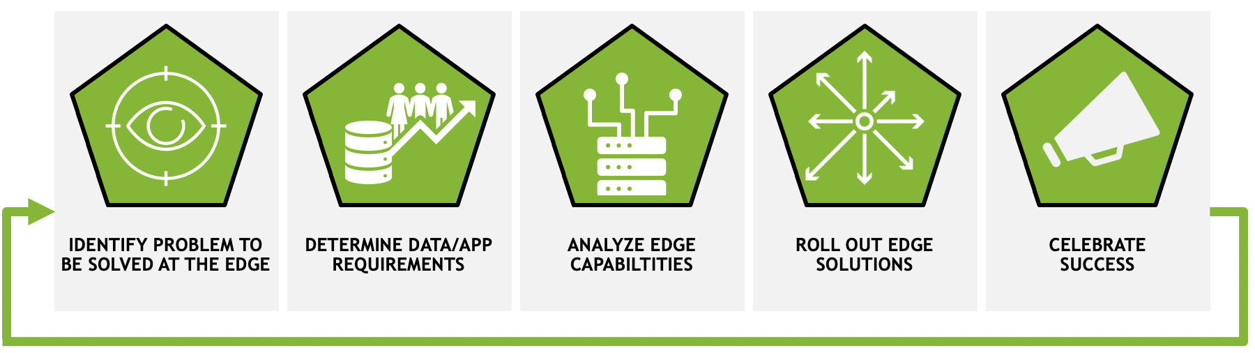
This post covers how network professionals can update their data center network infrastructure and protocol stack.

Data centers can be optimized by updating key network architectures in two ways: through networking technologies or operational efficiency in NetDevOps. In this post, we identify and evaluate technologies that you can apply to your network architecture to optimize your network.

We address five updates that you should consider for improving your data center:

  • Replace layer 2 VLANs with VXLAN.
  • Use Address Resolution Protocol (ARP) suppression to reduce broadcast propagation.
  • Replace multi-chassis link aggregation group (MLAG) with EVPN multihoming.
  • Handle traffic balancing with equal-cost multi-path (ECMP) routing and UCMP.
  • Accommodate traffic polarization with adaptive routing.

Replace VLANs with VXLANs

VXLAN is an overlay technology that uses encapsulation to allow a layer 2 overlay VLANs to span across layer 3 networks. Layer 2 networks have some inherent disadvantages:

  • Because they rely on spanning tree protocol (STP), the capability for redundancy and multiple paths is limited by the functionality of spanning tree.
  • They can only operate within one subnet, and redundancy is normally only limited to two devices due to MLAG.
  • Any path-level redundancy requires the Link Aggregation Control Protocol (LACP), the standard redundancy technology for ports.

VXLAN overcomes these deficiencies and allows the network operator to optimize on a layer 3 routed fabric. A layer 2 overlay can still be accomplished, but no longer requires spanning tree for control plane convergence due to the reliance of EVPN as the control plane.

EVPN exchanges MAC information through a BGP address family, instead of relying on the inefficiencies of broadcast flood and learn. Plus, VXLAN uses a 24-bit ID that can define up to 16 million virtual networks, whereas VLAN only has a 12-bit ID and is limited to 4094 virtual networks.

Use ARP suppression to reduce broadcast propagation

Broadcast traffic in data centers with VXLAN can be further optimized with ARP suppression. ARP suppression helps reduce traffic by using EVPN to proxy responses to ARP requests directly to clients from the ToR virtual tunnel end point (VTEP).

  • Without ARP suppression, all ARP requests are broadcast throughout the entire VXLAN fabric, sent to every VTEP that has a VNI for the network.
  • With ARP suppression enabled, MAC addresses learned over EVPN are passed down to the ARP control plane.

The leaf switch, which acts as the VTEP, responds directly back to the ARP requester through a proxy ARP reply.

Because the IP-to-MAC mappings are already communicated through the VXLAN control plane using EVPN type 2 messages, implementing ARP suppression enables optimization for faster resolution of the overlay control plane. It also reduces the amount of broadcast traffic in the fabric, as ARP suppression reduces the need for flooding ARP requests to every VTEP in the VXLAN infrastructure.

Replace MLAG with EVPN multihoming

Sometimes MLAG is still required in VXLAN environments for redundant host connectivity. EVPN multihoming is an opportunity to move off proprietary MLAG solutions that do not scale beyond one level of device redundancy.

As I mentioned earlier, VXLAN helps remove the need for back-to-back leaf-to-spine switch connections as required by MLAG. EVPN multihoming goes one step further and eliminates any need for MLAG in server-to-leaf connectivity.

Multihoming uses EVPN messages to communicate host connectivity, and it dynamically builds L2 adjacency to servers using host connectivity information. Where MLAG requires LAG IDs, multihoming uses Ethernet segment IDs. Interfaces are mapped to segments that act like logical connections to the same end host.

Additionally, moving to multihoming improves network vendor interoperability by using a protocol standard form of redundancy in the switch. Because multihoming uses BGP, an open standard protocol, any vendor implementing multihoming through the RFC specification can be part of the Ethernet segment.

ECMP and UCMP to handle traffic balancing

ECMP is a standard function in most layer 3 routing protocols where equal-cost routes are balanced across all available next-hop uplinks. Layer 2 control plane technologies like spanning-tree only allow equal-cost balancing by relying on external technologies like LACP.

ECMP is a native functionality in layer 3 routing, which enables you to get more efficiency out of your network devices.

There are cases where ECMP may lead to inefficient forwarding, specifically when doing a full layer 3 solution where point-to-point L3 links are used everywhere in the fabric, even to the host. In this case, you may want to balance traffic on a metric other than the number of links. UCMP can be useful here, as it uses BGP tags to create a distribution of traffic across hops to align better to your application distribution.

Accommodate traffic polarization with adaptive routing

Adaptive routing is an existing InfiniBand technology adopted by Ethernet switching. Adaptive routing monitors link bandwidth, link utilization, switch buffers, and ECN/PFC to understand when traffic on a specific path has become congested and would benefit from being dynamically rerouted through a less congested path.

Based on meeting these metric’s thresholds, the switch can redirect traffic from one egress interface to another egress interface in the ECMP group. This helps in fully leveraging all links on the switch equally, without the threat of polarization creating an inefficient traffic flow.

The goal of adaptive routing is to take any manual tuning intervention out of the hands of a network admin and let the infrastructure handle the optimizations for aggregate flow balancing.

Conclusion

In this post, we covered some concepts available in data center networking that can help you optimize a network infrastructure by focusing on the protocol stack and data plane. These optimizations provide better network virtualization, help reduce unnecessary control traffic on the infrastructure, and balance traffic across existing layer 1 links to fully use all the bandwidth available.

Categories
Misc

TensorFlow Releases TensorFlow v2.9 With New Features

TensorFlow has announced the release of version 2.9 just three months after the release of version 2.8. OneDNN, a novel model distribution API, and DTensor, an API for smooth data and model parallelism migration, are the key highlights of this release.

OneDNN

The oneDNN performance package was added to TensorFlow to improve Intel CPUs’ performance. The experimental support for oneDNN in TensorFlow has been available since version 2.5, delivering a four-fold increase in speed. Linux x86 packages and CPUs with neural-network-focused hardware capabilities like AVX512 VNNI, AVX512 BF16, AMX, and others found on Intel Cascade Lake and newer CPUs, oneDNN optimizations will be turned on by default.

Dtensor

Dtensor is a new API for disseminating models and is one of the most notable features of this edition. DTensorflow allows shifting from data parallelism to single program multiple data (SPMD) based model parallelism, including spatial partitioning. Model inputs that are too massive for a single device can now be trained using new tools available to developers. A model code can be utilized on CPU, GPU, or TPU, regardless of the device, because it is a device-agnostic API. This job likewise gets rid of the coordinator and instead uses the task’s local devices to control them all. Model scaling can be accomplished without affecting startup time.

TF Blog: https://blog.tensorflow.org/2022/05/whats-new-in-tensorflow-29.html

submitted by /u/No_Coffee_4638
[visit reddit] [comments]

Categories
Misc

Adding new block/inputs to non-sequential network

I am designing a progressive GAN and I have been stuck on an issue for a couple days now. I have successfully made my generator grow, but increasing the size of my discriminator is not that easy. in my discriminator, I decided to try implementing an ADA layer (like in the generator in StyleGAN3) However I have so far been unsuccessful in connecting the old layers with an input from a new block. The main problem is the non-sequential nature of the discriminator, as I need to give multiple inputs for the multiplication and addition layers. I will give the code to construct my discriminator, however I believe my code to add a block to the discriminator is wholly non-functioning, so that will not be included.

def construct_disc(label_dim=50): # Kernel Init init = tf.keras.initializers.HeUniform(seed=1) # Create Discriminator Inputs im_in = tf.keras.layers.Input(shape = (8,8,3)) lab_in = tf.keras.layers.Input(shape = (label_dim,)) # Style Vector Describer D = tf.keras.layers.Dense(3 * 3 * 3, activation=tf.keras.layers.LeakyReLU(alpha=0.2), kernel_initializer=init)(lab_in) D = tf.keras.layers.Dense(3 * 3 * 3, activation=tf.keras.layers.LeakyReLU(alpha=0.2), kernel_initializer=init)(D) D = tf.keras.layers.Dense(3 * 3 * 3, activation=tf.keras.layers.LeakyReLU(alpha=0.2), kernel_initializer=init)(D) # Conv Block Begins G = tf.keras.layers.Conv2D(128,1, padding = 'same', activation=tf.keras.layers.LeakyReLU(alpha=0.2), kernel_initializer=init)(im_in) G = tf.keras.layers.Conv2D(128,3, padding = 'same', activation = tf.keras.layers.LeakyReLU(alpha=0.2), kernel_initializer=init)(G) # Create Dense Style Interpreter (This Is Part Of The Block) W = tf.keras.layers.Dense(1)(D) W = W[:,:,tf.newaxis,tf.newaxis] B = tf.keras.layers.Dense(1)(D) B = B[:,:,tf.newaxis,tf.newaxis] G = tf.math.multiply(W, G) G = tf.add(G, B) G = tf.keras.layers.Conv2D(128,3, padding = 'same', activation = tf.keras.layers.LeakyReLU(alpha=0.2), kernel_initializer=init)(G) # Block Ends Here ^ G = tf.keras.layers.AveragePooling2D(2)(G) G = tf.keras.layers.Conv2D(128,3, padding = 'same', activation = tf.keras.layers.LeakyReLU(alpha=0.2), kernel_initializer=init)(G) G = tf.keras.layers.Flatten()(G) out = tf.keras.layers.Dense(1, activation='sigmoid', kernel_initializer=init)(G) model = tf.keras.Model([im_in, lab_in], out) # Compile Model opt = tf.keras.optimizers.Adam(lr=0.0002, beta_1=0.5) model.compile(loss=tf.keras.losses.BinaryCrossentropy(from_logits=True), optimizer=opt) return model 

submitted by /u/Yo1up
[visit reddit] [comments]