
 Linear regression is one of the simplest machine learning models out there. It is often the starting point not only for learning about data science but also for building quick and…
Linear regression is one of the simplest machine learning models out there. It is often the starting point not only for learning about data science but also for building quick and simple minimum viable products (MVPs), which then serve as benchmarks for more complex algorithms.
In general, linear regression fits a line (in two dimensions) or a hyperplane (in three and more dimensions) that best describes the linear relationship between the features and the target value. The algorithm also assumes that the probability distributions of the features are well-behaved; for example, they follow the Gaussian distribution.
Outliers are values that are located far outside of the expected distribution. They cause the distributions of the features to be less well-behaved. As a consequence, the model can be skewed towards the outlier values, which, as I’ve already established, are far away from the central mass of observations. Naturally, this leads to the linear regression finding a worse and more biased fit with inferior predictive performance.
It is important to remember that the outliers can be found both in the features and the target variable, and all the scenarios can worsen the performance of the model.
There are many possible approaches to dealing with outliers: removing them from the observations, treating them (capping the extreme observations at a reasonable value, for example), or using algorithms that are well-suited for dealing with such values on their own. This post focuses on these robust methods.
Setup
I use fairly standard libraries: numpy, pandas, scikit-learn. All the models I work with here are imported from the linear_model module of scikit-learn.
import numpy as np
import pandas as pd
import matplotlib.pyplot as plt
import seaborn as sns

from sklearn import datasets
from sklearn.linear_model import (LinearRegression, HuberRegressor,
                              	RANSACRegressor, TheilSenRegressor)
Data
Given that the goal is to show how different robust algorithms deal with outliers, the first step is to create a tailor-made dataset to show clearly the differences in the behavior. To do so, use the functionalities available in scikit-learn.
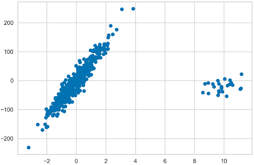
Start with creating a dataset of 500 observations, with one informative feature. With only one feature and the target, plot the data, together with the models’ fits. Also, specify the noise (standard deviation applied to the output) and create a list containing the coefficient of the underlying linear model; that is, what the coefficient would be if the linear regression model was fit to the generated data. In this example, the value of the coefficient is 64.6. Extract those coefficients for all the models and use them to compare how well they fit the data.
Next, replace the first 25 observations (5% of the observations) with outliers, far outside of the mass of generated observations. Bear in mind that the coefficient stored earlier comes from the data without outliers. Including them makes a difference.
N_SAMPLES = 500
N_OUTLIERS = 25

X, y, coef = datasets.make_regression(
	n_samples=N_SAMPLES,
	n_features=1,
	n_informative=1,
	noise=20,
	coef=True,
	random_state=42
)
coef_list = [["original_coef", float(coef)]]

# add outliers
np.random.seed(42)
X[:N_OUTLIERS] = 10 + 0.75 * np.random.normal(size=(N_OUTLIERS, 1))
y[:N_OUTLIERS] = -15 + 20 * np.random.normal(size=N_OUTLIERS)

plt.scatter(X, y);
Linear regression
Start with the good old linear regression model, which is likely highly influenced by the presence of the outliers. Fit the model to the data using the following example:
lr = LinearRegression().fit(X, y)
coef_list.append(["linear_regression", lr.coef_[0]])
Then prepare an object to use for plotting the fits of the models. The plotline_X object is a 2D array containing evenly spaced values within the interval dictated by the generated data set. Use this object for getting the fitted values for the models. It must be a 2D array, given it is the expected input of the models in scikit-learn. Then create a fit_df DataFrame in which to store the fitted values, created by fitting the models to the evenly spaced values.
plotline_X = np.arange(X.min(), X.max()).reshape(-1, 1)

fit_df = pd.DataFrame(
	index = plotline_X.flatten(),
	data={"linear_regression": lr.predict(plotline_X)}
)
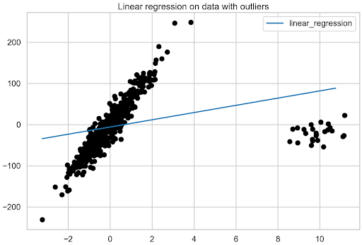
Having prepared the DataFrame, plot the fit of the linear regression model to the data with outliers.
fix, ax = plt.subplots()
fit_df.plot(ax=ax)
plt.scatter(X, y, c="k")
plt.title("Linear regression on data with outliers");
Figure 2 shows the significant impact that outliers have on the linear regression model.
The benchmark model has been obtained using linear regression. Now it is time to move toward robust regression algorithms.
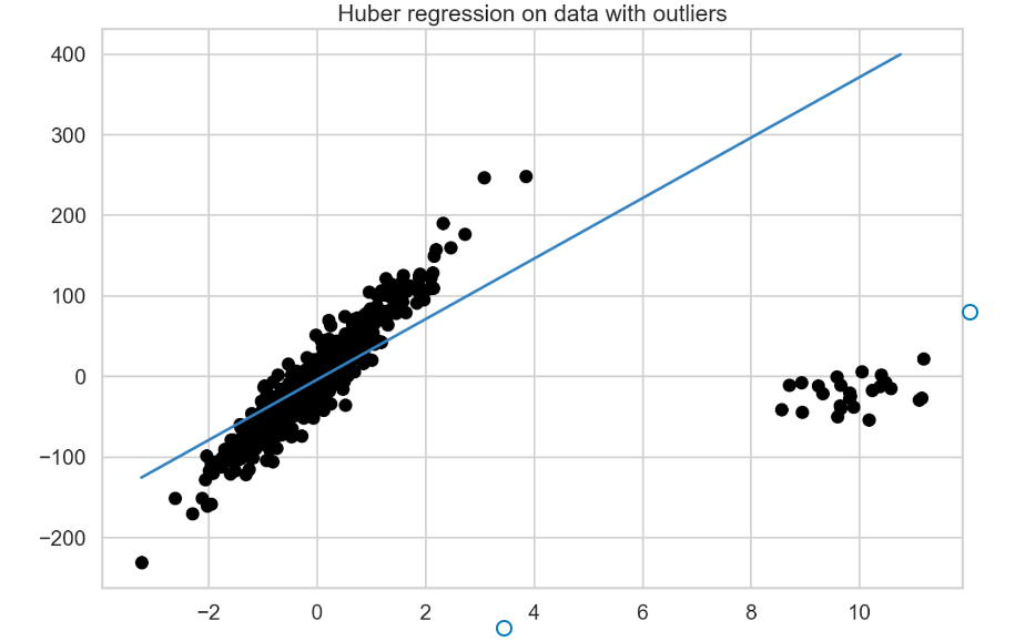
Huber regression
Huber regression is an example of a robust regression algorithm that assigns less weight to observations identified as outliers. To do so, it uses the Huber loss in the optimization routine. Here’s a better look at what is actually happening in this model.
Huber regression minimizes the following loss function:
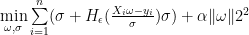
Where 


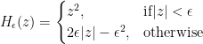
The Huber loss identifies outliers by considering the residuals, denoted by 

An inquisitive reader might notice that the first equation is similar to Ridge regression, that is, including the L2 regularization. The difference between Huber regression and Ridge regression lies in the treatment of outliers.
You might recognize this approach to loss functions from analyzing the differences between two of the popular regression evaluation metrics: mean squared error (MSE) and mean absolute error (MAE). Similar to what the Huber loss implies, I recommend using MAE when you are dealing with outliers, as it does not penalize those observations as heavily as the squared loss does.
Connected to the previous point is the fact that optimizing the squared loss results in an unbiased estimator around the mean, while the absolute difference leads to an unbiased estimator around the median. The median is much more robust to outliers than the mean, so expect this to provide a less biased estimate.
Use the default value of 1.35 for
For your own use cases, I recommend tuning the hyperparameters alpha and epsilon, using a method such as grid search.
Fit the Huber regression to the data using the following example:
huber = HuberRegressor().fit(X, y)
fit_df["huber_regression"] = huber.predict(plotline_X)
coef_list.append(["huber_regression", huber.coef_[0]])
Figure 3 presents the fitted model’s best fit line.
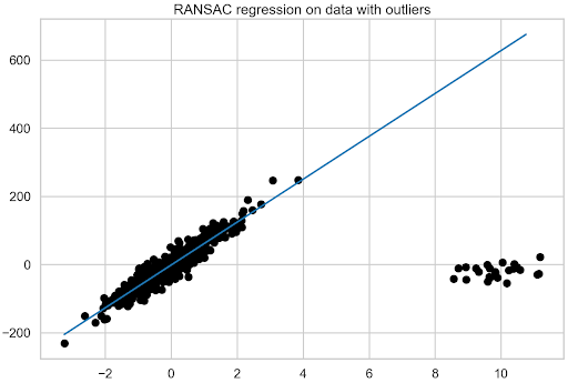
RANSAC regression
Random sample consensus (RANSAC) regression is a non-deterministic algorithm that tries to separate the training data into inliers (which may be subject to noise) and outliers. Then, it estimates the final model only using the inliers.
RANSAC is an iterative algorithm in which iteration consists of the following steps:
- Select a random subset from the initial data set.
- Fit a model to the selected random subset. By default, that model is a linear regression model; however, you can change it to other regression models.
- Use the estimated model to calculate the residuals for all the data points in the initial data set. All observations with absolute residuals smaller than or equal to the selected threshold are considered inliers and create the so-called consensus set. By default, the threshold is defined as the median absolute deviation (MAD) of the target values.
- The fitted model is saved as the best one if sufficiently many points have been classified as part of the consensus set. If the current estimated model has the same number of inliers as the current best one, it is only considered to be better if it has a better score.
The steps are performed iteratively either a maximum number of times or until a special stop criterion is met. Those criteria can be set using three dedicated hyperparameters. As I mentioned earlier, the final model is estimated using all inlier samples.
Fit the RANSAC regression model to the data.
ransac = RANSACRegressor(random_state=42).fit(X, y)
fit_df["ransac_regression"] = ransac.predict(plotline_X)
ransac_coef = ransac.estimator_.coef_
coef_list.append(["ransac_regression", ransac.estimator_.coef_[0]])
As you can see, the procedure for recovering the coefficient is a bit more complex, as it’s first necessary to access the final estimator of the model (the one trained using all the identified inliers) using estimator_. As it is a LinearRegression object, proceed to recover the coefficient as you did earlier. Then, plot the fit of the RANSAC regression (Figure 4).
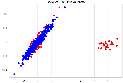
With RANSAC regression, you can also inspect the observations that the model considered to be inliers and outliers. First, check how many outliers the model identified in total and then how many of those that were manually introduced overlap with the models’ decision. The first 25 observations of the training data are all the outliers that have been introduced.
inlier_mask = ransac.inlier_mask_
outlier_mask = ~inlier_mask
print(f"Total outliers: {sum(outlier_mask)}")
print(f"Outliers you added yourself: {sum(outlier_mask[:N_OUTLIERS])} / {N_OUTLIERS}")
Running the example prints the following summary:
Total outliers: 51
Outliers you added yourself: 25 / 25
Roughly 10% of data was identified as outliers and all the observations introduced were correctly classified as outliers. It’s then possible to quickly visualize the inliers compared to outliers to see the remaining 26 observations flagged as outliers.
plt.scatter(X[inlier_mask], y[inlier_mask], color="blue", label="Inliers")
plt.scatter(X[outlier_mask], y[outlier_mask], color="red", label="Outliers")
plt.title("RANSAC - outliers vs inliers");
Figure 5 shows that the observations located farthest from the hypothetical best-fit line of the original data are considered outliers.
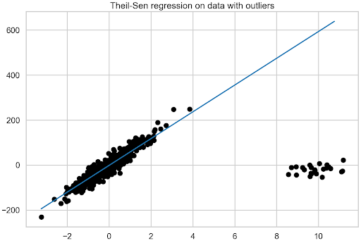
Theil-Sen regression
The last of the robust regression algorithms available in scikit-learn is the Theil-Sen regression. It is a non-parametric regression method, which means that it makes no assumption about the underlying data distribution. In short, it involves fitting multiple regression models on subsets of the training data and then aggregating the coefficients at the last step.
Here’s how the algorithm works. First, it calculates the least square solutions (slopes and intercepts) on subsets of size p (hyperparameter n_subsamples) created from all the observations in the training set X. If you calculate the intercept (it is optional), then the following condition must be satisfied p >= n_features + 1. The final slope of the line (and possibly the intercept) is defined as the (spatial) median of all the least square solutions.
A possible downside of the algorithm is its computational complexity, as it can consider a total number of least square solutions equal to n_samples choose n_subsamples, where n_samples is the number of observations in X. Given that this number can quickly explode in size, there are a few things that can be done:
- Use the algorithm only for small problems in terms of the number of samples and features. However, for obvious reasons, this might not always be feasible.
- Tune the
n_subsampleshyperparameter. A lower value leads to higher robustness to outliers at the cost of lower efficiency, while a higher value leads to lower robustness and higher efficiency. - Use the
max_subpopulationhyperparameter. If the total value ofn_samples choose n_subsamplesis larger thanmax_subpopulation, the algorithm only considers a stochastic subpopulation of a given maximal size. Naturally, using only a random subset of all the possible combinations leads to the algorithm losing some of its mathematical properties.
Also, be aware that the estimator’s robustness decreases quickly with the dimensionality of the problem. To see how that works out in practice, estimate the Theil-Sen regression using the following example:
theilsen = TheilSenRegressor(random_state=42).fit(X, y)
fit_df["theilsen_regression"] = theilsen.predict(plotline_X)
coef_list.append(["theilsen_regression", theilsen.coef_[0]])
Comparison of the models
So far, three robust regression algorithms have been fitted to the data containing outliers and the individual best fit lines have been identified. Now it is time for a comparison.
Start with the visual inspection of Figure 7. To show too many lines, the fit line of the original data is not printed. However, it is quite easy to imagine what it looks like, given the direction of the majority of the data points. Clearly, the RANSAC and Theil-Sen regressions have resulted in the most accurate best fit lines.
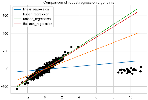
To be more precise, look at the estimated coefficients. Table 1 shows that the RANSAC regression results in the fit closest to the one of the original data. It is also interesting to see how big of an impact the 5% of outliers had on the regular linear regression’s fit.
| model | coefficient | |
| 0 | original_coef |
64.59 |
| 1 | linear_regression |
8.77 |
| 2 | huber_regression |
37.52 |
| 3 | ransac_regression |
62.85 |
| 4 | theilsen_regression |
59.49 |
You might ask which robust regression algorithm is the best? As is often the case, the answer is, “It depends.” Here are some guidelines that might help you find the right model for your specific problem:
- In general, robust fitting in a high-dimensional setting is difficult.
- In contrast to Theil-Sen and RANSAC, Huber regression is not trying to completely filter out the outliers. Instead, it lessens their effect on the fit.
- Huber regression should be faster than RANSAC and Theil-Sen, as the latter ones fit on smaller subsets of the data.
- Theil-Sen and RANSAC are unlikely to be as robust as the Huber regression using the default hyperparameters.
- RANSAC is faster than Theil-Sen and it scales better with the number of samples.
- RANSAC should deal better with large outliers in the y-direction, which is the most common scenario.
Taking all the preceding information into consideration, you might also empirically experiment with all three robust regression algorithms and see which one fits your data best.
You can find the code used in this post in my /erykml GitHub repo. I look forward to hearing from you in the comments.