Joseph Fraunhofer was a 19th-century pioneer in optics who brought together scientific research with industrial applications. Fast forward to today and Germany’s Fraunhofer Society — Europe’s largest R&D organization — is setting its sights on the applied research of key technologies, from AI to cybersecurity to medicine. Its Fraunhofer IML unit is aiming to push Read article >
Data is the fuel that makes artificial intelligence run. Training machine learning and AI systems requires data. And the quality of datasets has a big impact on the systems’ results. But compiling quality real-world data for AI and ML can be difficult and expensive. That’s where synthetic data comes in. The guest for this week’s Read article >
In the NVIDIA Studio celebrates the Open Broadcaster Software (OBS) Studio’s 10th anniversary and its 28.0 software release. Plus, popular streamer WATCHHOLLIE shares how she uses OBS and a GeForce RTX 3080 GPU in a single-PC setup to elevate her livestreams.
The increasing adoption of cloud-native workloads is causing a significant shift in infrastructure architecture to support next-generation applications such as…
The increasing adoption of cloud-native workloads is causing a significant shift in infrastructure architecture to support next-generation applications such as AI and big data. Infrastructure must evolve to provide composability and flexibility using virtualization, containers, or bare metal servers.
Traditional software-defined infrastructure provides flexibility but suffers from performance and scalability limitations, as up to 30% of server CPU cores may be consumed by workloads such as networking, storage, and security.
VMware saw this as an opportunity to enhance vSphere infrastructure and reengineered it to take a hardware-based, disaggregated approach. The infrastructure software stack is now tightly coupled to the hardware stack. The result is VMware vSphere Distributed Services Engine (VMware Project Monterey), which integrates closely with the NVIDIA BlueField DPU to provide an evolutionary architectural approach for data center, cloud, and edge. It addresses the changing requirements of next-gen and cloud-native workloads.
To help organizations test the benefits of vSphere on BlueField DPUs, NVIDIA LaunchPad has curated a lab with exclusive access to live demonstrations and self-paced learning. The lab is designed to provide your IT team with deep, practical experience in a hosted environment before starting an on-premises deployment.
vSphere Distributed Services Engine
vSphere Distributed Services Engine is a software-defined and hardware-accelerated architecture for VMware’s Cloud Foundation. It provides a breakthrough solution that supports virtualization, containers, and scalable management.
The BlueField DPU offloads, accelerates, and isolates the infrastructure workloads, allowing the server CPUs to focus on core applications and revenue-generating tasks. The integration of VMware vSphere and NVIDIA BlueField simplifies building a cloud-ready infrastructure, while providing a consistent service quality in multi-cloud environments.
VMware enables workload composability and portability that supports multi-cloud. At the same time, BlueField handles critical networking, storage, security, and management, including telemetry tasks, freeing up the CPUs to run business and tenant applications. The BlueField DPU also provides security isolation by running firewall, key management, and IDS/IPS on its Arm cores, in a separate domain from the applications.
NVIDIA LaunchPad
LaunchPad gives you access to dedicated hardware and software through a remote lab, so that IT teams can walk through the entire process of deploying and managing a vSphere on BlueField DPUs. The lab is designed to provide your IT team with deep, practical experience in a hosted environment before starting your on-premises deployment.
Background
To understand why this is important, start by looking at how modern applications have changed. Modern applications are driving many underlying hardware infrastructure requirements, including
Increased networking traffic that creates performance and scale challenges
Hardware acceleration requirements that drive significant operational complexities
A lack of a clear definition of the traditional data center perimeter, which intensifies the need for new security models.
We are seeing that modern applications require more server CPU cycles. As the application requirements for compute continue to grow, increased infrastructure requirements for CPU cycles compete with application requirements.
Specialized data processing units (DPUs) have been developed to offload, accelerate and isolate CPU networking, storage, security, and management tasks. With DPUs, organizations free up server-CPU cycles for core application processing, which accelerates job completion time over a robust zero-trust data center infrastructure.
Selected functions that used to run on the core CPU are offloaded, accelerated, and isolated on BlueField to support new possibilities, including the following:
Improved performance for application and infrastructure services
Enhanced visibility, application security, and observability
Isolated security capabilities
Enhanced data center efficiency and reduced enterprise, edge, and cloud costs
Next steps
VMware vSphere is leading the shift to advanced hybrid-cloud data center architectures, which benefit from the hypervisor and accelerated software-defined networking, security, and storage. With access to vSphere on BlueField DPU preconfigured clusters, you can explore the evolution of VMware Cloud Foundation and take advantage of the disruptive hardware capabilities of servers equipped with BlueField DPUs.
In the machine learning and MLOps world, GPUs are widely used to speed up model training and inference, but what about the other stages of the workflow like ETL…
In the machine learning and MLOps world, GPUs are widely used to speed up model training and inference, but what about the other stages of the workflow like ETL pipelines or hyperparameter optimization?
Within the RAPIDS data science framework, ETL tools are designed to have a familiar look and feel to data scientists working in Python. Do you currently use Pandas, NumPy, Scikit-learn, or other parts of the PyData stack within your KubeFlow workflows? If so, you can use RAPIDS to accelerate those parts of your workflow by leveraging the GPUs likely already available in your cluster.
In this post, I demonstrate how to drop RAPIDS into a KubeFlow environment. You start with using RAPIDS in the interactive notebook environment and then scale beyond your single container to use multiple GPUs across multiple nodes with Dask.
Optional: Installing KubeFlow with GPUs
This post assumes you are already somewhat familiar with Kubernetes and KubeFlow. To explore how you can use GPUs with RAPIDS on KubeFlow, you need a KubeFlow cluster with GPU nodes. If you already have a cluster or are not interested in KubeFlow installation instructions, feel free to skip ahead.
KubeFlow is a popular machine learning and MLOps platform built on Kubernetes for designing and running machine learning pipelines, training models, and providing inference services.
KubeFlow also provides a notebook service that you can use to launch an interactive Jupyter server in your Kubernetes cluster and a pipeline service with a DSL library, written in Python, to create repeatable workflows. Tools for adjusting hyperparameters and running a model inference server are also accessible. This is essentially all the tooling that you need for building a robust machine learning service.
For this post, you use Google Kubernetes Engine (GKE) to launch a Kubernetes cluster with GPU nodes and install KubeFlow onto it, but any KubeFlow cluster with GPUs will do.
Creating a Kubernetes cluster with GPUs
First, use the gcloud CLI to create a Kubernetes cluster.
$ gcloud container clusters create rapids-gpu-kubeflow
  --accelerator type=nvidia-tesla-a100,count=2 --machine-type a2-highgpu-2g
  --zone us-central1-c --release-channel stable
Note: Machines with GPUs have certain limitations which may affect your workflow. Learn more at https://cloud.google.com/kubernetes-engine/docs/how-to/gpus
Creating cluster rapids-gpu-kubeflow in us-central1-c...
Cluster is being health-checked (master is healthy)...
Created
kubeconfig entry generated for rapids-gpu-kubeflow.
NAME             	LOCATION   	MASTER_VERSION	MASTER_IP   	MACHINE_TYPE   NODE_VERSION  	NUM_NODES  STATUS
rapids-gpu-kubeflow  us-central1-c  1.21.12-gke.1500  34.132.107.217  a2-highgpu-2g  1.21.12-gke.1500  3      	RUNNING
With this command, you’ve launched a GKE cluster called rapids-gpu-kubeflow. You’ve specified that it should use nodes of type a2-highgpu-2g, each with two A100 GPUs.
KubeFlow also requires a stable version of Kubernetes, so you specified that along with the zone in which to launch the cluster.
Then, install KubeFlow by cloning the KubeFlow manifests repo, checking out the latest release, and applying them.
$ git clone https://github.com/kubeflow/manifests
$ cd manifests
$ git checkout v1.5.1 # Or whatever the latest release is
$ while ! kustomize build example | kubectl apply -f -; do echo "Retrying to apply resources"; sleep 10; done
After all the resources have been created, KubeFlow still has to bootstrap itself on your cluster. Even after this command finishes, things may not be ready yet. This can take upwards of 15 minutes.
Eventually, you should see a full list of KubeFlow services in the kubeflow namespace.
After all your pods are in a Running state, port forward the KubeFlow web user interface, and access it in your browser.
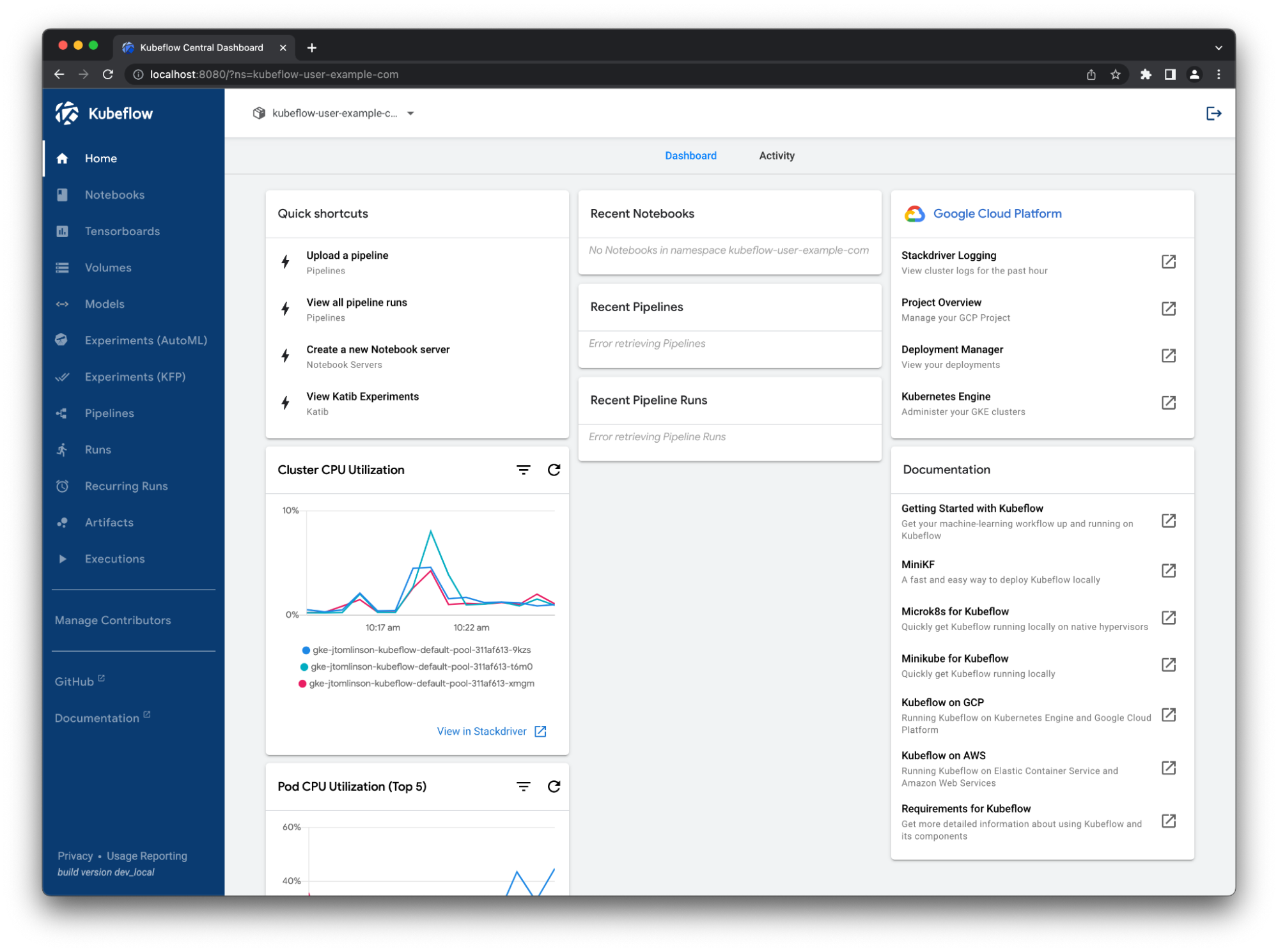
Navigate to 127.0.0.1:8080 and log in with the default credentials user@example.com and 12341234. Then, you should see the KubeFlow dashboard (Figure 1).
Before launching your cluster, you must create a configuration profile that is important for when you start using Dask later. To do this, apply the following manifest:
Now, choose a RAPIDS version to use. Typically, you want to choose the container image for the latest release. The default CUDA version installed on GKE Stable is 11.4, so choose that. As of version 11.5 and later, it won’t matter as they will be backward compatible. Copy the container image name from the installation command:
Scroll down to Configurations, check the configure dask dashboard option, scroll to the bottom of the page, and then choose Launch. You should see it starting up in your list of notebooks. The RAPIDS container images are packed full of amazing tools, so this step can take a little while.
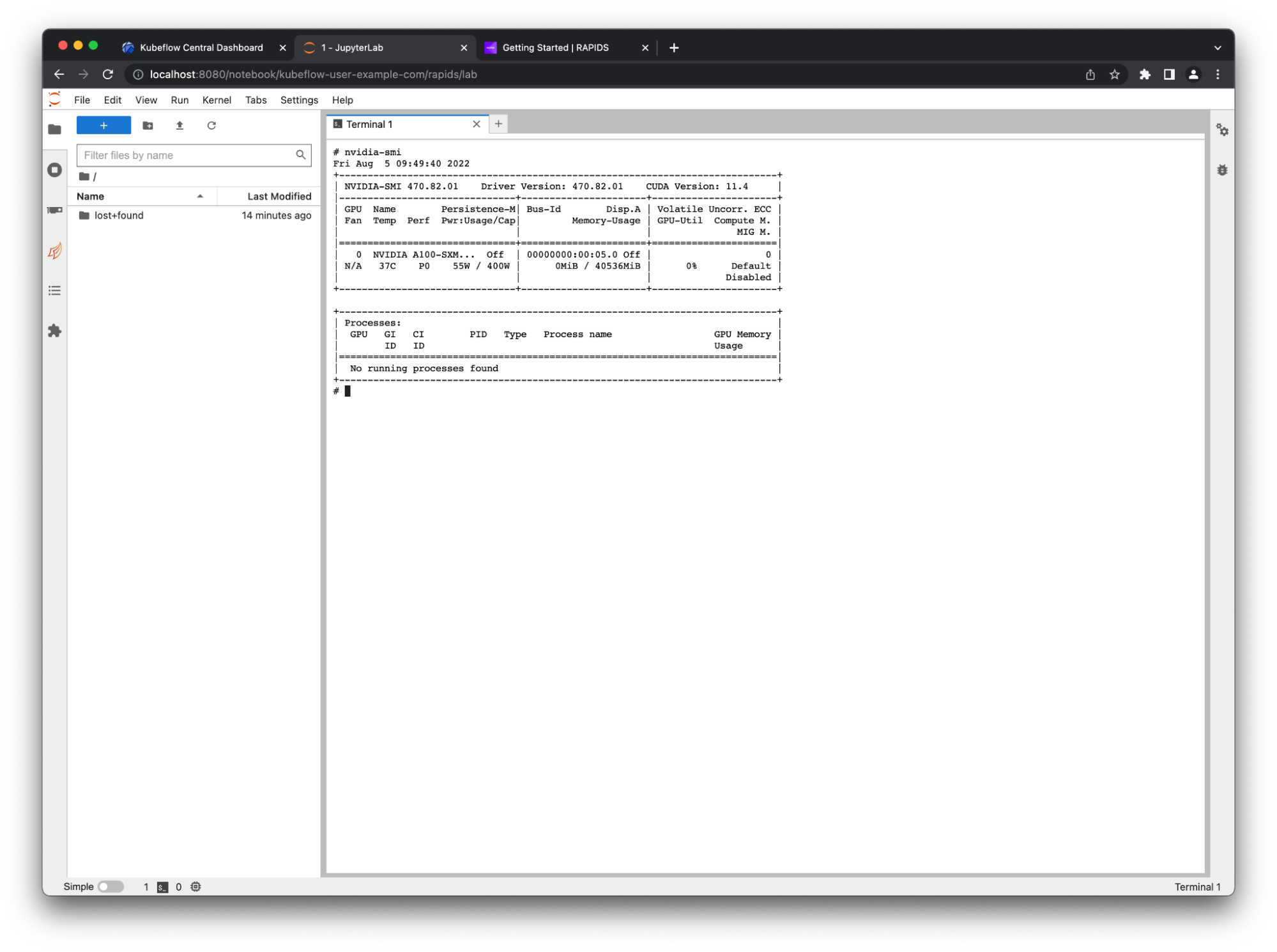
When the notebook is ready, to launch Jupyter, choose Connect. Verify that everything works okay by opening a terminal window and running nvidia-smi (Figure 2).
Figure 2. The nvidia-smi command is a great way to check that your GPU is set up
Success! Your A100 GPU is being passed through into your notebook container.
The RAPIDS container that you chose also comes with some example notebooks, which you can find in /rapidsai/notebooks. Make a quick symbolic link to these from your home directory so that you can navigate using the file explorer on the left:
ln -s /rapids/notebooks /home/jovyan/notebooks.
Navigate to those example notebooks and explore all the libraries that RAPIDS offers. For example, ETL developers that use pandas should check out the cuDF notebooks for examples of accelerated DataFrames.
Scaling your RAPIDS workflows
Many RAPIDS libraries also support scaling out your computations onto multiple GPUs spread over many nodes for added acceleration. To do this, use Dask, an open-source Python library for distributed computing.
To use Dask, create a scheduler and some workers to perform your calculations. These workers also need GPUs and the same Python environment as the notebook session. Dask has an operator for Kubernetes that you can use to manage Dask clusters on your KubeFlow cluster, so install that now.
Installing the Dask Kubernetes operator
To install the operator, you create the operator itself and its associated custom resources. For more information, see Installing in the Dask documentation.
In the terminal window that you used to create your KubeFlow cluster, run the following commands:
Verify that your resources were applied successfully by listing your Dask clusters. You shouldn’t expect to see any but the command should succeed.
$ kubectl get daskclusters
No resources found in default namespace.
You can also check that the operator pod is running and ready to launch new Dask clusters.
$ kubectl get pods -A -l application=dask-kubernetes-operator
NAMESPACE       NAME                                        READY   STATUS    RESTARTS   AGE
dask-operator   dask-kubernetes-operator-775b8bbbd5-zdrf7   1/1     Running   0          74s
Lastly, make sure that your notebook session can create and manage the Dask custom resources. To do this, edit the kubeflow-kubernetes-edit cluster role that gets applied to your notebook pods. Add a new rule to the rules section for this role to allow everything in the kubernetes.dask.org API group.
Now, create DaskCluster resources in Kubernetes to launch all the necessary pods and services for your cluster to work. You can do this in YAML through the Kubernetes API if you like but for this post, use the Python API from the notebook session.
Back in the Jupyter session, create a new notebook and install the dask-kubernetes package that you need for launching your clusters.
!pip install dask-kubernetes
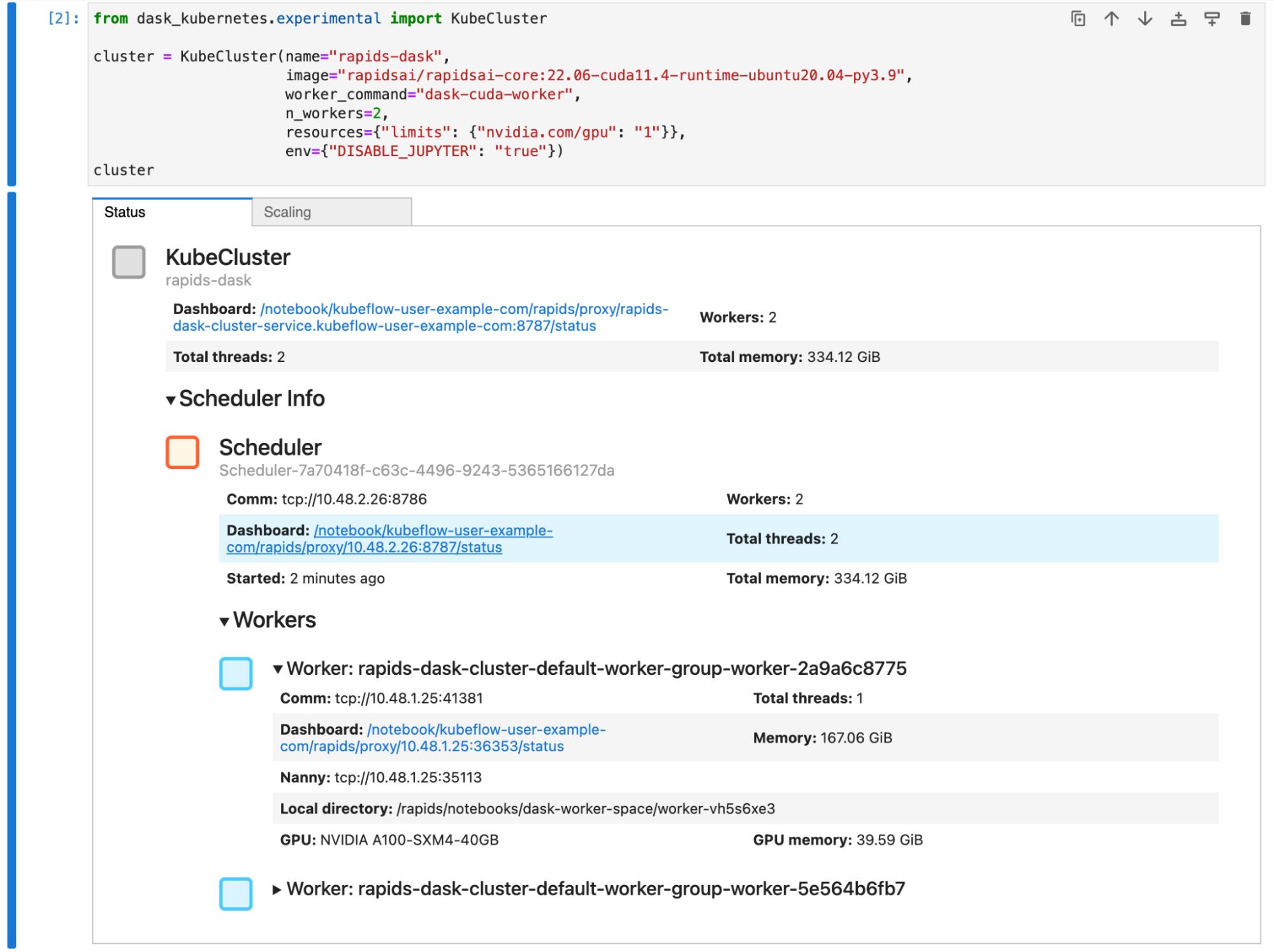
Next, create a Dask cluster using the KubeCluster class. Confirm that you set the container image to match the one you chose for your notebook environment and set the number of GPUs to 1. You also tell the RAPIDS container not to start Jupyter by default and run the Dask command instead.
This can take a similar amount of time to starting up the notebook container, as it also has to pull the RAPIDS Docker image.
Figure 3 shows that you have a Dask cluster with two workers, and that each worker has an A100 GPU, the same as your Jupyter session.
Figure 3. Dask has many useful widgets that you can view in your notebook to show the status of your cluster
You scale this cluster up and down with either the scaling tab in the widget in Jupyter or by calling cluster.scale(n) to set the number of workers, and therefore the number of GPUs.
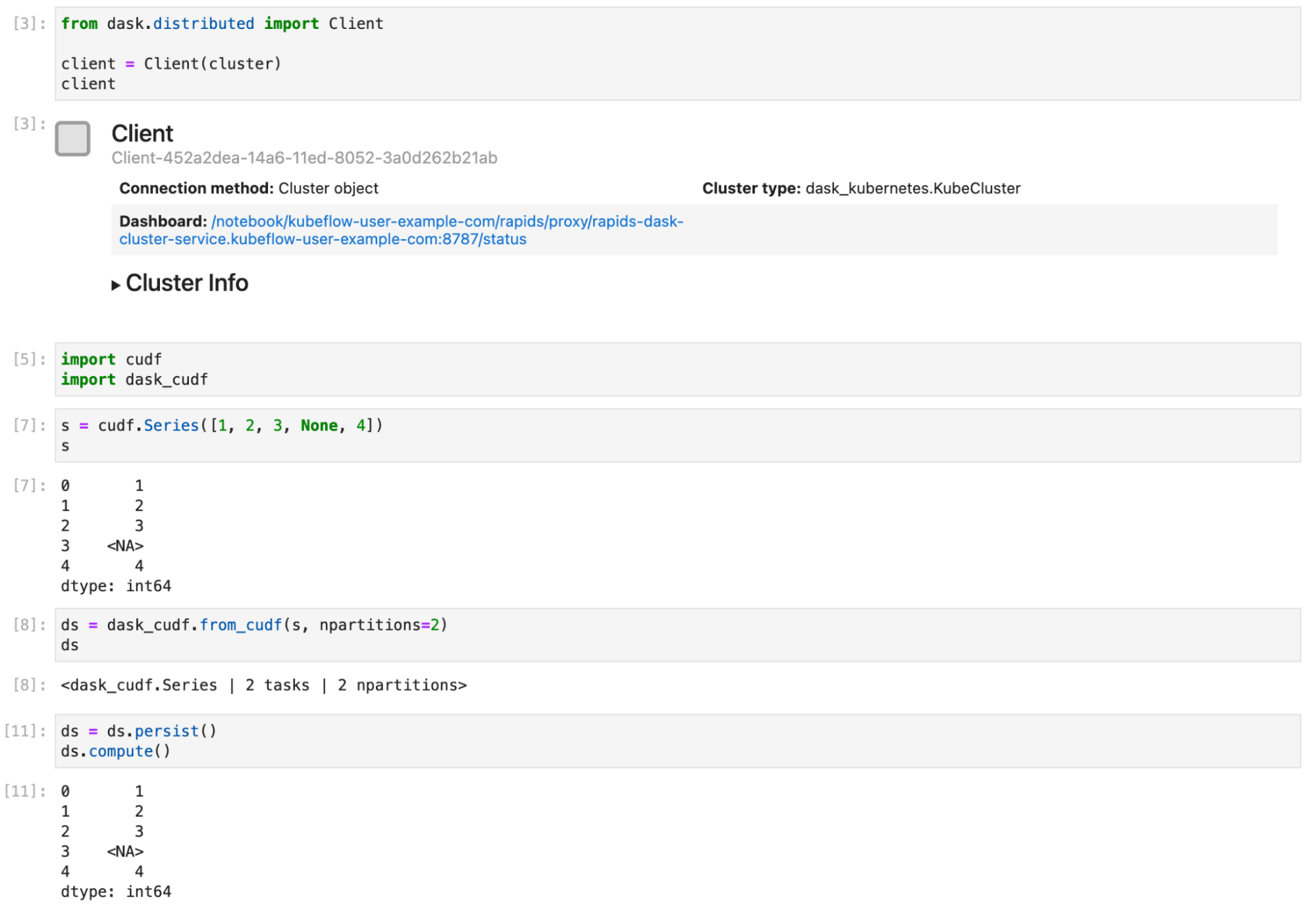
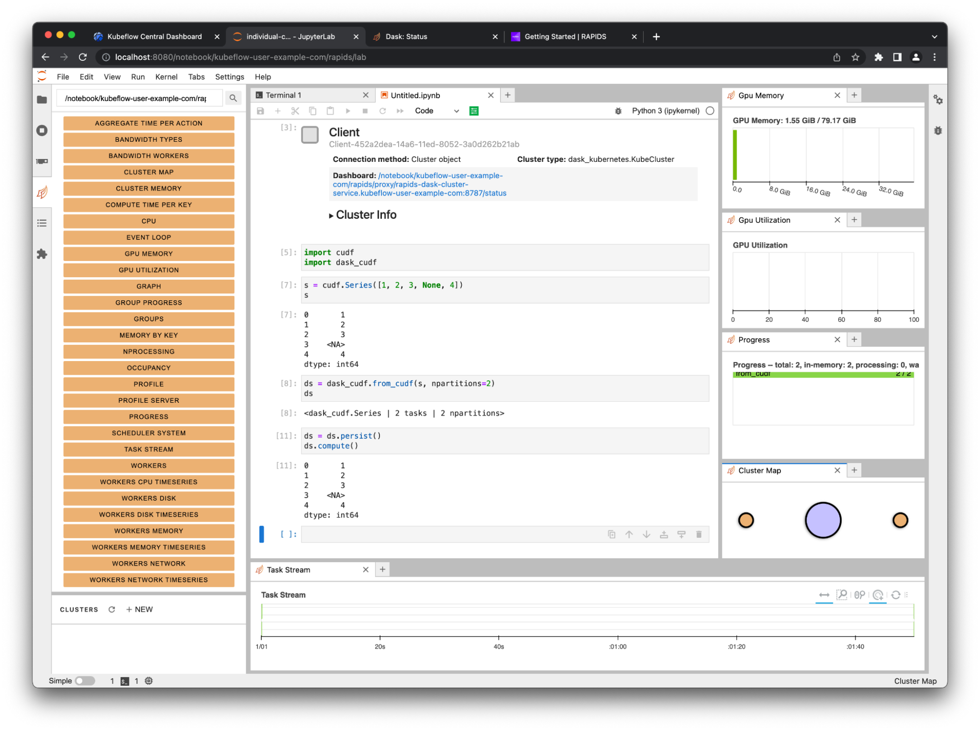
Now, connect a Dask client to your cluster. From that point on, any RAPIDS libraries that support Dask, such as dask_cudf, use your cluster to distribute your computation over all your GPUs. Figure 4 shows a short example of creating a Series object and distributing it with Dask.
Figure 4. Create a cuDF DataFrame, distributed it with Dask, then perform a computation and get the results
Accessing the Dask dashboard
At the beginning of this section, you added an extra config file with some options for the Dask dashboard. These options are necessary to enable you to access the dashboard running in the scheduler pod on your Kubernetes cluster from your Jupyter environment.
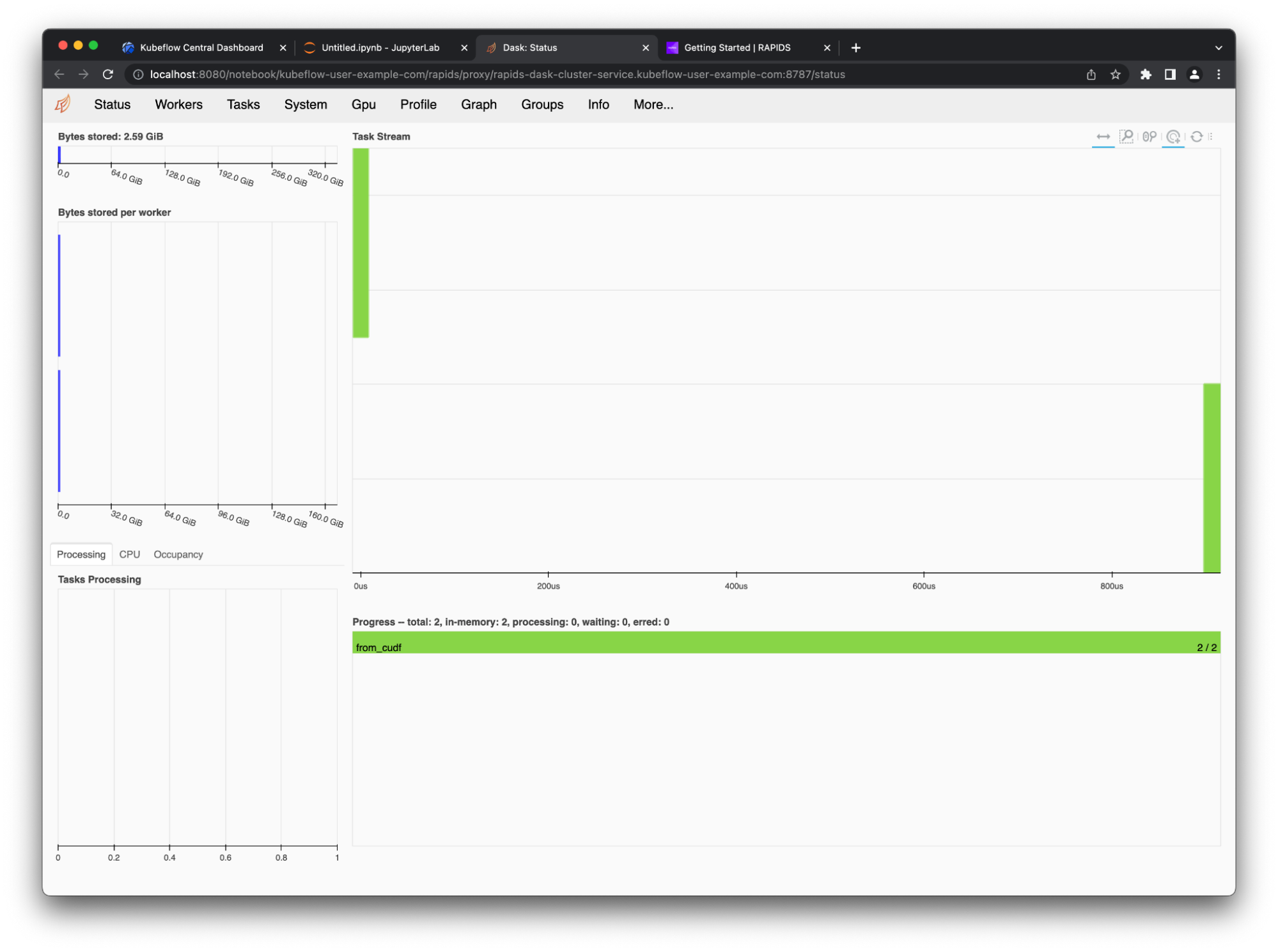
You may have noticed that the cluster and client widgets both had links to the dashboard. Select these links to open the dashboard in a new tab (Figure 5).
Figure 5. Dask dashboard with the from_cudf call
You can also use the Dask JupyterLab extension to view various plots and stats about your Dask cluster right in JupyterLab.
On the Dask tab on the left, choose the search icon. This connects JupyterLab to the dashboard through the client in your notebook. Select the various plots and arrange them in JupyterLab by dragging the tabs around.
Figure 6. The Dask dashboard has many useful plots, including some dedicated GPU metrics like memory use and utilization
If you followed along with this post, clean up all the created resources by deleting the GKE cluster created at the start.
RAPIDS integrates seamlessly with KubeFlow enabling you to use your GPU resources in the ETL stages of your workflows, as well during training and inference.
You can either drop the RAPIDS environment straight into the KubeFlow notebooks service for single-node work or use the Dask Operator for Kubernetes from KubeFlow Pipelines to scale that workload onto many nodes and GPUs.
For more information about using RAPIDS, see the following resources:
Crafted by AI for AI, GPUNet is a class of convolutional neural networks designed to maximize the performance of NVIDIA GPUs using NVIDIA TensorRT. Built using…
Crafted by AI for AI, GPUNet is a class of convolutional neural networks designed to maximize the performance of NVIDIA GPUs using NVIDIA TensorRT.
Built using novel neural architecture search (NAS) methods, GPUNet demonstrates state-of-the-art inference performance up to 2x faster than EfficientNet-X and FBNet-V3.
The NAS methodology helps build GPUNet for a wide range of applications such that deep learning engineers can directly deploy these neural networks depending on the relative accuracy and latency targets.
GPUNet NAS design methodology
Efficient architecture search and deployment-ready models are the key goals of the NAS design methodology. This means little to no interaction with the domain experts and efficient use of cluster nodes for training potential architecture candidates. Most important is that the generated models are deployment-ready.
Crafted by AI
Finding the best performing architecture search for a target device can be time-consuming. NVIDIA built and deployed a novel NAS AI agent that efficiently makes the tough design choices required to build GPUNets that beat the current SOTA models by a factor of 2x.
This NAS AI agent automatically orchestrates hundreds of GPUs in the Selene supercomputer without any intervention from the domain experts.
Optimized for NVIDIA GPU using TensorRT
GPUNet picks up the most relevant operations required to meet the target model accuracy with related TensorRT inference latency cost, promoting GPU-friendly operators (for example, larger filters) over memory-bound operators (for example, fancy activations). It delivers the SOTA GPU latency and the accuracy on ImageNet.
Deployment-ready
The GPUNet reported latencies include all the performance optimization available in the shipping version of TensorRT, including fused kernels, quantization, and other optimized paths. Built GPUNets are ready for deployment.
Building a GPUNet: An end-to-end NAS workflow
At a high level, the neural architecture search (NAS) AI agent is split into two stages:
Categorizing all possible network architectures by the inference latency.
Using a subset of these networks that fit within the latency budget and optimizing them for accuracy.
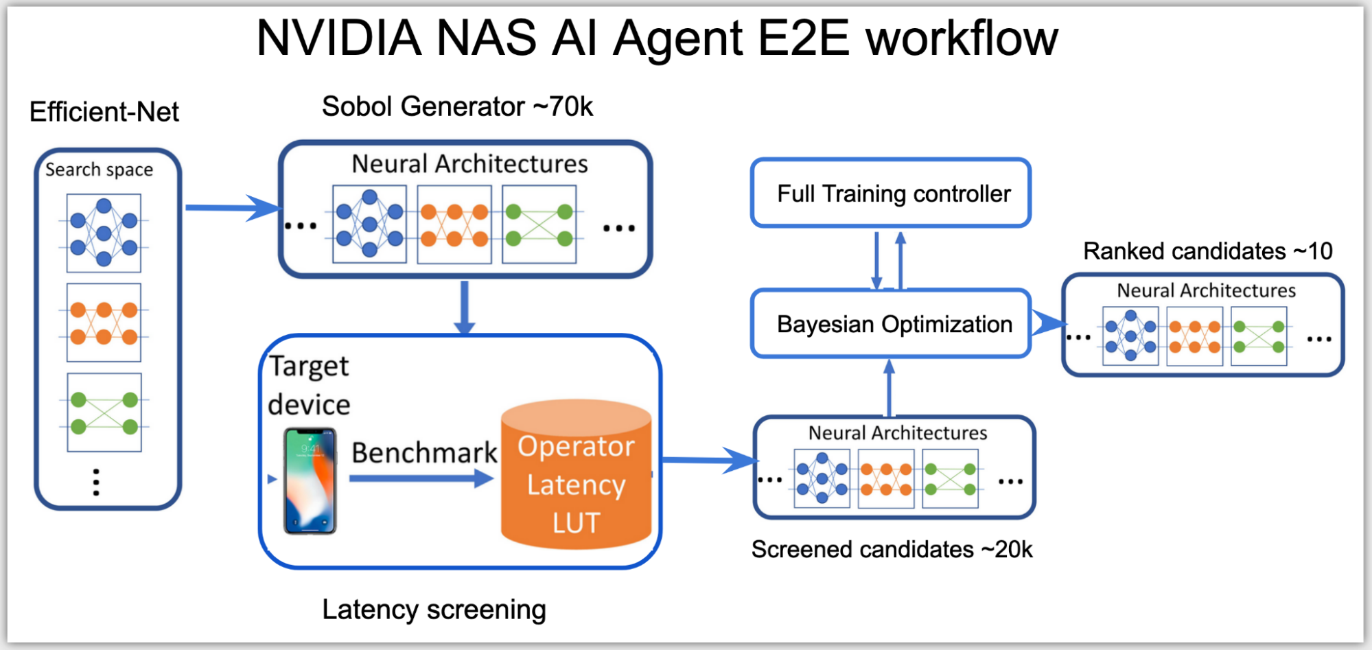
In the first stage, as the search space is high-dimensional, the agent uses Sobol sampling to distribute the candidates more evenly. Using the latency look-up table, these candidates are then categorized into a subsearch space, for example, a subset of networks with total latency under 0.5 msecs on NVIDIA V100 GPUs.
The inference latency used in this stage is an approximate cost, calculated by summing up the latency of each layer from the latency lookup table. The latency table uses input data shape and layer configurations as keys to look up the related latency on the queried layer.
In the second stage, the agent sets up Bayesian optimization loss function to find the best performing higher accuracy network within the latency range of the subspace:
Figure 2. NVIDIA NAS AI Agent End-to-End workflow
The AI agent uses a client-server distributed training controller to perform NAS simultaneously across multiple network architectures. The AI agent runs on one server node, proposing and training network candidates that run on several client nodes on the cluster.
Based on the results, only the promising network architecture candidates that meet both the accuracy and the latency targets of the target hardware get ranked, resulting in a handful of best-performing GPUNets that are ready to be deployed on NVIDIA GPUs using TensorRT.
GPUNet model architecture
The GPUNet model architecture is an eight-stage architecture using EfficientNet-V2 as the baseline architecture.
The search space definition includes searching on the following variables:
Type of operations
Number of strides
Kernel size
Number of layers
Activation function
IRB expansion ratio
Output channel filters
Squeeze excitation (SE)
Table 1 shows the range of values for each variable in the search space.
Table 1. Value ranges for search space variables
Stage
Type
Stride
Kernel
Layers
Activation
ER
Filters
SE
0
Conv
2
[3,5]
1
[R,S]
[24, 32, 8]
1
Conv
1
[3,5]
[1,4]
[R,S]
[24, 32, 8]
2
F-IRB
2
[3,5]
[1,8]
[R,S]
[2, 6]
[32, 80, 16]
[0, 1]
3
F-IRB
2
[3,5]
[1,8]
[R,S]
[2, 6]
[48, 112, 16]
[0, 1]
4
IRB
2
[3,5]
[1,10]
[R,S]
[2, 6]
[96, 192, 16]
[0, 1]
5
IRB
1
[3,5]
[0,15]
[R,S]
[2, 6]
[112, 224, 16]
[0, 1]
6
IRB
2
[3,5]
[1,15]
[R,S]
[2, 6]
[128, 416, 32]
[0, 1]
7
IRB
1
[3,5]
[0,15]
[R,S]
[2, 6]
[256, 832, 64]
[0, 1]
8
Conv1x1 & Pooling & FC
The first two stages search for the head configurations using convolutions. Inspired by EfficientNet-V2, the second and third stages use Fused-IRB. Fused-IRBs result in higher latency though, so in stages 4 to 7 these are replaced by IRBs.
The column Layers show the range of layers in the stage. For example, [1, 10] in stage 4 means that the stage can have 1 to 10 IRBs. The column Filters shows the range of output channel filters for the layers in the stage. This search space also tunes the expansion ratio (ER), activation types, kernel sizes, and the Squeeze Excitation (SE) layer inside the IRB/Fused-IRB.
Finally, the dimensions of the input image are searched from 224 to 512, at the step of 32.
Each GPUNet candidate build from the search space is encoded into a 41-wide integer vector (Table 2).
Table 2. The encoding scheme of networks in the search space
Stage
Type
Hyperparameters
Length
Resolution
[Resolution]
1
0
Conv
[#Filters]
1
1
Conv
[Kernel, Activation, #Layers]
3
2
Fused-IRB
[#Filters, Kernel, E, SE, Act, #Layers]
6
3
Fused-IRB
[#Filters, Kernel, E, SE, Act, #Layers]
6
4
IRB
[#Filters, Kernel, E, SE, Act, #Layers]
6
5
IRB
[#Filters, Kernel, E, SE, Act, #Layers]
6
6
IRB
[#Filters, Kernel, E, SE, Act, #Layers]
6
7
IRB
[#Filters, Kernel, E, SE, Act, #Layers]
6
At the end of the NAS search, the returned ranked candidates is a list of these best-performing encodings, which are in turn the best-performing GPUNets.
Summary
All ML practitioners are encouraged to read the CVPR 2022 GPUNet paper, with related GPUNet training code on the NVIDIA/DeepLearningExamples GitHub repo, and run inference on the colab instance on available cloud GPUs. GPUNet inference is also available on the PyTorch hub. The colab run instance uses the GPUNet checkpoints hosted on the NGC hub. These checkpoints have varying accuracy and latency tradeoffs, which can be applied based on the requirement of the target application.
Clinical applications for AI are improving digital surgery, helping to reduce errors, provide consistency, and enable surgeon augmentations that were previously…
Clinical applications for AI are improving digital surgery, helping to reduce errors, provide consistency, and enable surgeon augmentations that were previously unimaginable.
In endoscopy, a minimally invasive procedure used to examine the interior of an organ or cavity of a body, AI and accelerated computing are enabling better detection rates and visibility.
Endoscopists can investigate symptoms, make a diagnosis, and treat patients by cauterizing a bleeding blood vessel, for example. There are numerous forms of endoscopy, many of them focused on gastroenterological diseases that affect the digestive tract.
Colonoscopy, one of the most common forms of gastrointestinal endoscopy, is essential for catching colorectal cancer, a disease that the American Cancer Society predicts will affect over 150,000 people in 2022.
With the assistance of AI, surgeries like endoscopy are becoming safer and more consistent while reducing surgeon workload. The tasks being augmented with machine learning algorithms include labeling, clearing surgical smoke, classifying airway diseases, identifying airway sizes, identifying lesions and diseased tissue, and auto-calculating the best physical routes for instruments.
To enable these clinical applications, technical algorithms are being developed for specific tasks:
Organ segmentation for detection and automatic measurements
Tool tracking
Tissue type identification
Optical flow
Legion classification
Enhancing and processing video streams
In endoscopy, the task of enhancing and processing video streams is key to augmenting surgeon technical skills. This includes tasks of endoscopic image denoising, anomaly object detection, and anomaly measurements, as well as the streaming tasks of ingesting high-resolution and high-bandwidth data.
To implement AI and accomplish these tasks, developers must address numerous challenges in the medical device development process such as:
Ingesting high resolution, high-bandwidth data streams
Running AI inference with a low-latency budget
Finding flexible sensor and data I/O options
Building a distributed compute platform from edge to data center to cloud
Adopting new deep learning algorithms
Today, most developers have to build individual solutions every time they have to solve a problem or workflow bottleneck. NVIDIA Clara Holoscan is a development platform with compute for AI workloads. With workloads such as enhanced visualization and automatic anomaly detection, you can easily customize solutions for various challenges.
Having an accelerated platform to iterate and integrate AI into endoscopy workflows gives you a low-risk, low-cost approach for adding augmentations to your existing endoscopy systems.
Whether deploying latency-sensitive, real-time tasks on the edge or analytic and summarization tasks to the cloud, NVIDIA Clara Holoscan offloads complexity, allowing you to quickly build custom AI solutions to improve endoscopy.
Endoscopy AI sample application on NVIDIA Clara Holoscan
Reference applications can provide an easy starting point if you’re looking to build custom applications for medical devices. The NVIDIA Clara Holoscan SDK includes a sample AI-enabled endoscopy application as a template for reusing components and app graphs in existing applications to build custom AI pipelines.
The endoscopy AI sample application has the end-to-end functionality of GXF, a modular and extensible framework to build high-performance applications. GXF provides support for devices that interface withAJA with an HDMI input. Its deep learning model can perform object detection and tool tracking in real time on an endoscopy video stream.
Several features are used to minimize the overall latency:
GPUDirect RDMA video data transfer to eliminate the overhead of copying to or from system memory.
TensorRT runtime for optimized AI Inference and speed-up.
CUDA and OpenGL interoperability, which provides efficient resource sharing on the GPU for visualization.
For more information about the endoscopy AI sample application, its hardware and software reference architecture on NVIDIA Clara Holoscan, as well as the path to production, see the Clara Holoscan Endoscopy whitepaper.
Featured image
An endoscopy image from a gallbladder surgery showing an AI-powered frame-by-frame tool identification and tracking. Image courtesy of Research Group Camma, IHU Strasbourg, and University of Strasbourg.
Reinventing enterprise computing for the modern era, VMware CEO Raghu Raghuram Tuesday announced the availability of the VMware vSphere 8 enterprise workload platform running on NVIDIA DPUs, or data processing units, an initiative formerly known as Project Monterey. Placing the announcement in context, Raghuram and NVIDIA founder and CEO Jensen Huang discussed how running VMware Read article >
Multi-Instance GPU (MIG) is an important feature of NVIDIA H100, A100, and A30 Tensor Core GPUs, as it can partition a GPU into multiple instances. Each…
Multi-Instance GPU (MIG) is an important feature of NVIDIA H100, A100, and A30 Tensor Core GPUs, as it can partition a GPU into multiple instances. Each instance has its own compute cores, high-bandwidth memory, L2 cache, DRAM bandwidth, and media engines such as decoders.
This enables multiple workloads or multiple users to run workloads simultaneously on one GPU to maximize the GPU utilization, with guaranteed quality of service (QoS). A single A30 can be partitioned into up to four MIG instances to run four applications in parallel.
This post walks you through how to use MIG on A30 from partitioning MIG instances to running deep learning applications on MIG instances at the same time.
A30 MIG profiles
By default, MIG mode is disabled on the A30. You must enable MIG mode and then partition the A30 before any CUDA workloads can be run on the partitioned GPU. To partition the A30, create GPU instances and then create corresponding compute instances.
A GPU instance is a combination of GPU slices and GPU engines (DMAs, NVDECs, and so on). A GPU slice is the smallest fraction of the GPU that combines a single GPU memory slice and a single streaming multiprocessor (SM) slice.
Within a GPU instance, the GPU memory slices and other GPU engines are shared, but the SM slices could be further subdivided into compute instances. A GPU instance provides memory QoS.
You can configure an A30 with 24 GB of memory to have:
One GPU instance, with 24 GB of memory
Two GPU instances, each with 12 GB of memory
Three GPU instances, one with 12 GB of memory and two with 6 GB
Four GPU instances, each with 6 GB of memory
A GPU instance could be further divided into one or more compute instances depending on the size of the GPU instance. A compute instance contains a subset of the parent GPU instance’s SM slices. The compute instances within a GPU instance share memory and other media engines. However, each compute instance has dedicated SM slices.
For example, you could divide an A30 into four GPU instances, each having one compute instance, or divide an A30 into two GPU instances, each having two compute instances. Although both partitions result in four compute instances that can run four applications at the same time, the difference is that memory and other engines are isolated at the GPU instance level, not at the compute instance level. Therefore, if you have more than one user to share an A30, it is better to create different GPU instances for different users to guarantee QoS.
Table 1 provides an overview of the supported MIG profiles on A30, including the five possible MIG configurations that show the number of GPU instances and the number of GPU slices in each GPU instance. It also shows how hardware decoders are partitioned among the GPU instances.
Config
GPC Slice #0
GPC Slice #1
GPC Slice #2
GPC Slice #3
OFA
NVDEC
NVJPG
P2P
GPU Direct RDMA
1
4
1
4
1
No
Supported MemBW proportional to the size of the instance
2
2
2
0
2+2
0
No
3
2
1
1
0
2+1+1
0
No
4
1
1
2
0
1+1+2
0
No
5
1
1
1
1
0
1+1+1+1
0
No
Table 1. The MIG profiles supported on A30
GPC (graphics processing cluster) or slice represents a grouping of the SMs, caches, and memory. The GPC maps directly to the GPU instance. OFA (Optical Flow Accelerator) is an engine on the GA100 architecture on which A100 and A30 are based. Peer-to-peer (P2P) is disabled.
Table 2 provides profile names of the supported MIG instances on A30, and how the memory, SMs, and L2 cache are partitioned among the MIG profiles. The profile names for MIG can be interpreted as its GPU instance’s SM slice count and its total memory size in GB. For example:
MIG 2g.12gb means that this MIG instance has two SM slices and 12 GB of memory
MIG 4g.24gb means that this MIG instance has four SM slices and 24 GB of memory
By looking at the SM slice count of 2 or 4 in 2g.12gb or 4g.24gb, respectively, you know that you can divide that GPU instance into two or four compute instances. For more information, see Partitioning in the MIG User Guide.
Profile
Fraction of memory
Fraction of SMs
Hardware units
L2 cache size
Number of instances available
MIG 1g.6gb
1/4
1/4
0 NVDECs /0 JPEG /0 OFA
1/4
4
MIG 1g.6gb+me
1/4
1/4
1 NVDEC /1 JPEG /1 OFA
1/4
1 (A single 1g profile can include media extensions)
MIG 2g.12gb
2/4
2/4
2 NVDECs /0 JPEG /0 OFA
2/4
2
MIG 4g.24gb
Full
4/4
4 NVDECs /1 JPEG /1 OFA
Full
1
Table 2. Supported GPU instance profiles on A30 24GB
MIG 1g.6gb+me: me means media extensions to get access to the video and JPEG decoders when creating the 1g.6gb profile.
MIG instances can be created and destroyed dynamically. Creating and destroying does not impact other instances, so it gives you the flexibility to destroy an instance that is not being used and create a different configuration.
Manage MIG instances
Automate the creation of GPU instances and compute instances with the MIG Partition Editor (mig-parted) tool or by following the nvidia-smi mig commands in Getting Started with MIG.
The mig-parted tool is highly recommended, as it enables you to easily change and apply the configuration of the MIG partitions each time without issuing a sequence of nvidia-smi mig commands. Before using the tool, you must install the mig-parted tool following the instructions or grab the prebuilt binaries from the tagged releases.
Here’s how to use the tool to partition the A30 into four MIG instances of the 1g.6gb profile. First, create a sample configuration file that can then be used with the tool. This sample file includes not only the partitions discussed earlier but also a customized configuration, custom-config, that partitions GPU 0 to four 1g.6gb instances and GPU 1 to two 2g.12gb instances.
Next, apply the all-1g.6gb configuration to partition the A30 into four MIG instances. If MIG mode is not already enabled, then mig-parted enables MIG mode and then creates the partitions:
You can easily pick other configurations or create your own customized configurations by specifying the MIG geometry and then using mig-parted to configure the GPU appropriately.
After creating the MIG instances, now you are ready to run some workloads!
Deep learning use case
You can run multiple deep learning applications simultaneously on MIG instances. Figure 1 shows four MIG instances (four GPU instances, each with one compute instance), each running a model for deep learning inference, to get the most out of a single A30 for four different tasks at the same time.
For example, you could have ResNet50 (image classification) on instance one, EfficientDet (object detection) on instance two, BERT (language model) on instance three, and FastPitch (speech synthesis) on instance four. This example can also represent four different users sharing the A30 at the same time with ensured QoS.
Figure 1. A single A30 with four MIG instances running four models for inference simultaneously
Performance analysis
To analyze the performance improvement of A30 with and without MIG enabled, we benchmarked the fine-tuning time and throughput of the BERT PyTorch model for SQuAD (question answering) in three different scenarios on A30 (with and without MIG), also on T4.
A30 four MIG instances, each has a model, in total four models fine-tuning simultaneously
A30 MIG mode disabled, four models fine-tuning in four containers simultaneously
A30 MIG mode disabled, four models fine-tuning in serial
T4 has four models fine-tuning in serial
Fine-tune BERT base, PyTorch, SQuAD, BS=4
1
2
3
4
Result
A30 MIG: four models on four MIG devices simultaneously
Time (sec)
5231.96
5269.44
5261.70
5260.45
5255.89 (Avg)
Sequences/sec
33.88
33.64
33.69
33.70
134.91(Total)
A30 No MIG: four models in four containers simultaneously
Time (sec)
7305.49
7309.98
7310.11
7310.38
7308.99 (Avg)
Sequences/sec
24.26
24.25
24.25
24.25
97.01(Total)
A30 No MIG: four models in serial
Time (sec)
1689.23
1660.59
1691.32
1641.39
6682.53 (Total)
Sequences/sec
104.94
106.75
104.81
108.00
106.13(Avg)
T4: four models in serial
Time (sec)
4161.91
4175.64
4190.65
4182.57
16710.77(total)
Sequences/sec
42.59
42.45
42.30
42.38
42.43(Avg)
Table 3. Inference time (sec) and throughput (sequences/sec) for the four cases
To run this example, use the instructions in Quick Start Guide and Performance benchmark sections in the NVIDIA/DeepLearningExamples GitHub repo.
Based on the experimental results in Table 3, A30 with four MIG instances shows the highest throughput and shortest fine-tuning time for four models in total.
Speedup of total fine-tuning time for A30 with MIG:
1.39x compared to A30 No MIG on four models simultaneously
1.27x compared to A30 No MIG on four models in serial
3.18x compared to T4
Throughput of A30 MIG
1.39x compared to A30 No MIG on four models simultaneously
1.27x compared to A30 No MIG on four models in serial
3.18x compared to T4
Fine-tuning on A30 with four models simultaneously without MIG can also achieve high GPU utilization, but the difference is that there is no hardware isolation such as MIG provides. It incurs overhead from context switching and leads to lower performance compared to using MIG.
What’s next?
Built on the latest NVIDIA Ampere Architecture to accelerate diverse workloads such as AI inference at scale, A30 MIG mode enables you to get the most out of a single GPU and serve multiple users at the same time with quality of service.
No one likes standing around and waiting for the bus to arrive, especially when you need to be somewhere on time. Wouldn’t it be great if you could predict…
No one likes standing around and waiting for the bus to arrive, especially when you need to be somewhere on time. Wouldn’t it be great if you could predict when the next bus is due to arrive?
At the beginning of this year, Armenian developer Edgar Gomtsyan had some time to spare, and he puzzled over this very question. Rather than waiting for a government entity to implement a solution, or calling the bus dispatchers to try to confirm bus arrival times, he developed his own solution. Based on machine learning, it predicts bus arrival times with a high degree of accuracy.
As it happens, Gomtsyan’s apartment faces the street where a bus stop is located. To track the arrival and departure of buses, he mounted a small security camera on his balcony that uses image recognition software. “Like in any complex problem, to come to an effective solution, the problem was separated into smaller parts,” Gomtsyan said.
His solution uses a Dahua IP camera. For video processing, he initially used Vertex AI which can be used for image and object detection, classification, and other needs. Due to concerns about possible network and electricity issues, he eventually decided to process the video stream details locally using an NVIDIA Jetson Nano. You can access various libraries and trained models in the jetson-inference repo on GitHub.
The Real Time Streaming Protocol (RTSP) connected details from the camera’s video stream to the Jetson Nano. Then, using imagenet for classification and one of the pretrained models in the GitHub repo, Gomtsyan was able to get basic classifications for the stream right away.
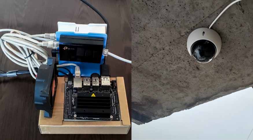
Figure 1. The router with PoE adapter and Jetson Nano (left) and the mounted Dahua IP camera (right)
For the training geeks in the crowd, things start to get interesting at this point. Using the pretrained model, Gomtsyan used his setup to take a screenshot from the video stream every time it detected a bus. His first model was ready with around 100 pictures.
But, as Gomtsyan admits, “To say that things were perfect at first would be wrong.” It became obvious to him that he needed more pictures to increase the precision of the model output. Once he had 300 pictures, “the system got better and better,” he said.
When he first shared the results of this project, his model had been trained with more than 1,300 pictures, and it detects both arriving and departing buses—even in different weather conditions. He was also able to distinguish between scheduled buses from buses that happened to arrive randomly. His model now includes three classes of image detection: an arriving bus, background (everything that is not a scheduled bus), and a departing bus.
As an example, if an ‘arriving bus’ class prediction is greater than or equal to 92% for 15 frames, then it records the arrival time to a local CSV file.
To improve the data collected, his system takes a screenshot from the stream every time it detects a bus. This helps with both future model retraining and finding false-positive detections.
Further, to overcome the limitations of storing the CSV file data locally, Gomtsyan opted to store the data in BigQuery using the Google IoT service. As he notes, storing the data in the cloud “gives a more flexible and sustainable solution that will cater to future enhancements.”
He used the information collected to create a model that will predict when the next bus will arrive using the Vertex AI regression service. Gomtsyan recommends watching the video below to learn how to set up the model.
Video 1. Learn how to build and train ML models with Vertex AI
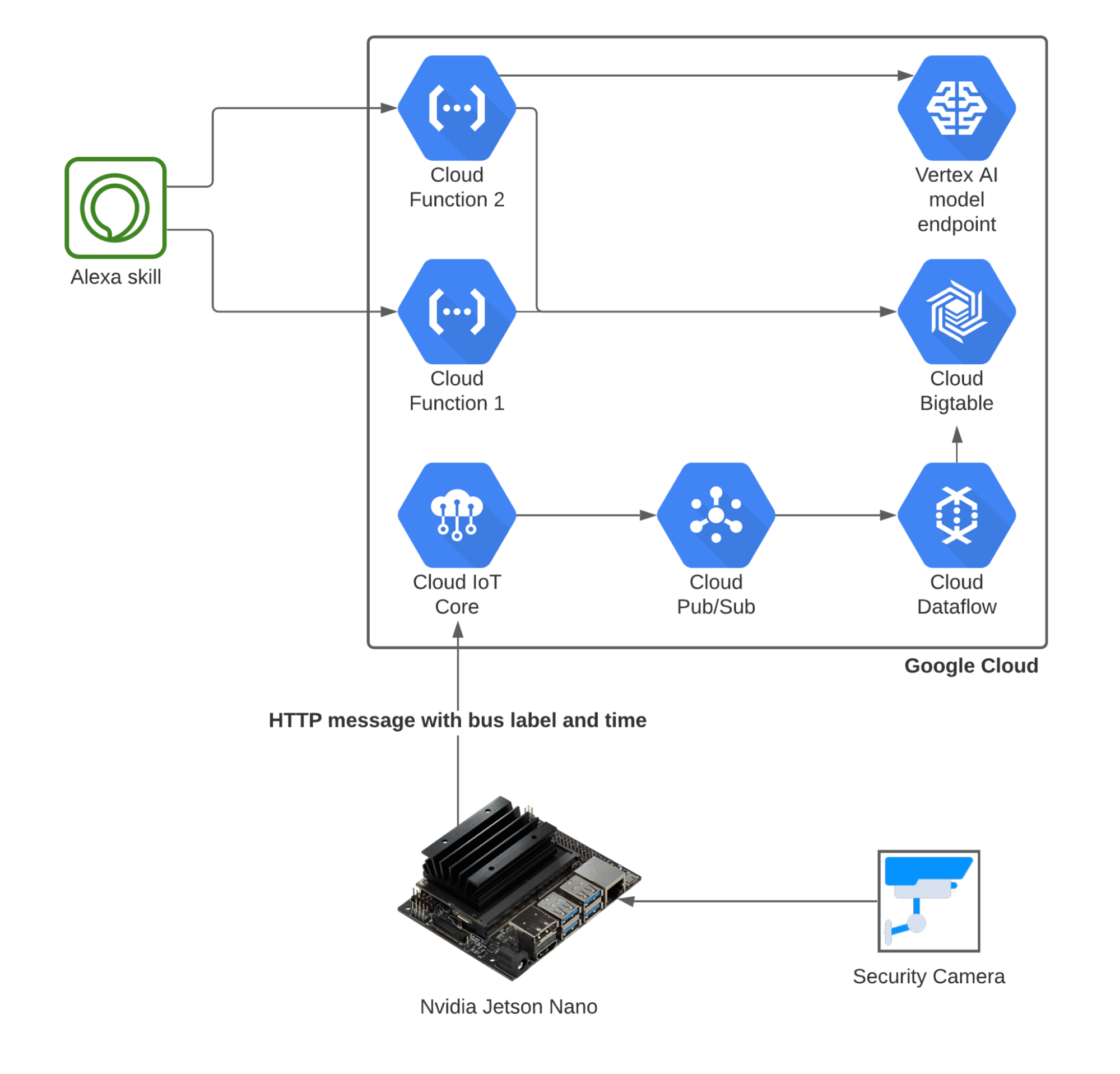
With a working model up and running, Gomtsyan needed an interface to let him know when the next bus should arrive. Rather than a website, he opted to use an IoT-based voice assistant. He originally planned to use Google Assistant for this purpose, but it was more challenging than expected. He instead used Alexa Skill, which is Amazon’s voice assistant tool. He created an Alexa Skill which queries respective cloud functions based on commands spoken to an Alexa speaker in his apartment.
Figure 2. The final architecture for Gomtsyan’s model
And while the predictions aren’t perfect, Gomtsyan has ideas for future enhancements that could help to improve the accuracy of the predicted bus arrival times, including traffic congestion data along the bus route. He is also considering using solar panels to power the system and make it autonomous, and introducing DevOps practices.
Gomtsyan developed this project to learn and challenge himself. Using his project documentation, other developers can replicate—and perhaps improve upon—his work. In the end, he hopes this bus prediction project will encourage others to pursue their ideas, “no matter how crazy, hard, or impossible they sound.”

 The increasing adoption of cloud-native workloads is causing a significant shift in infrastructure architecture to support next-generation applications such as…
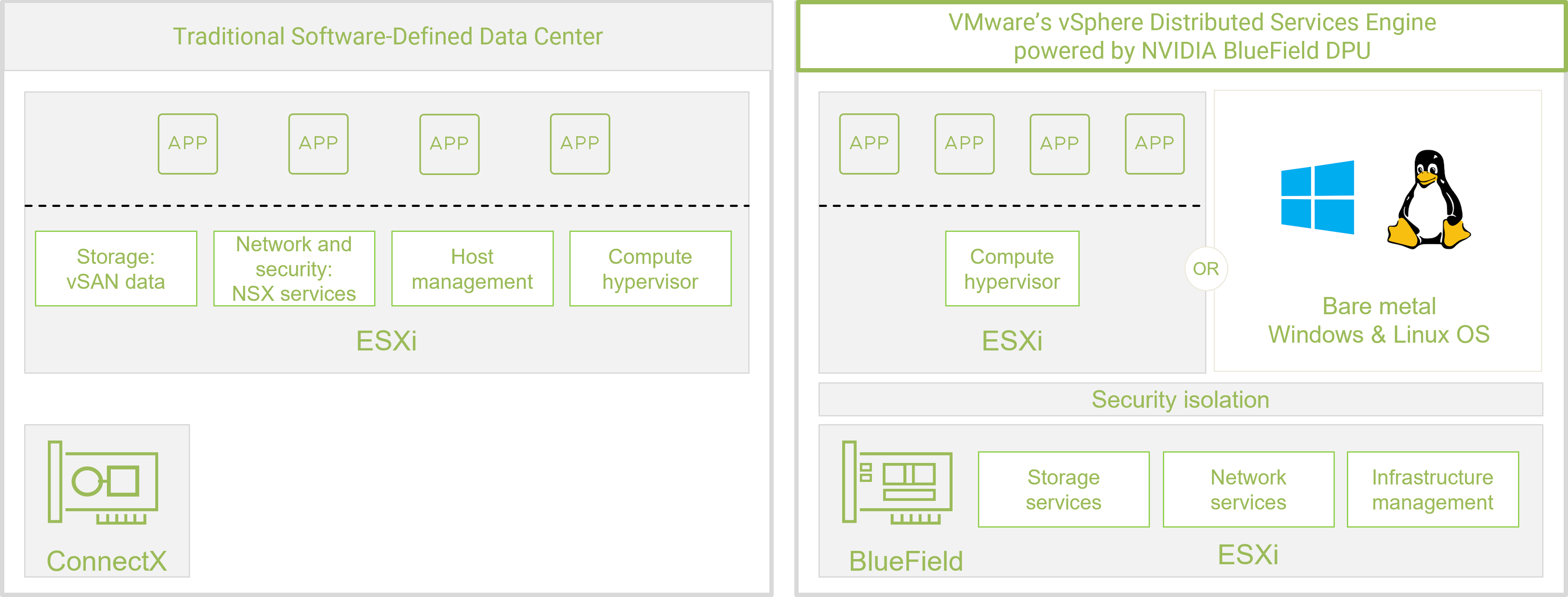
 In the machine learning and MLOps world, GPUs are widely used to speed up model training and inference, but what about the other stages of the workflow like ETL…
 Crafted by AI for AI, GPUNet is a class of convolutional neural networks designed to maximize the performance of NVIDIA GPUs using NVIDIA TensorRT. Built using…
 Clinical applications for AI are improving digital surgery, helping to reduce errors, provide consistency, and enable surgeon augmentations that were previously…
 Multi-Instance GPU (MIG) is an important feature of NVIDIA H100, A100, and A30 Tensor Core GPUs, as it can partition a GPU into multiple instances. Each…
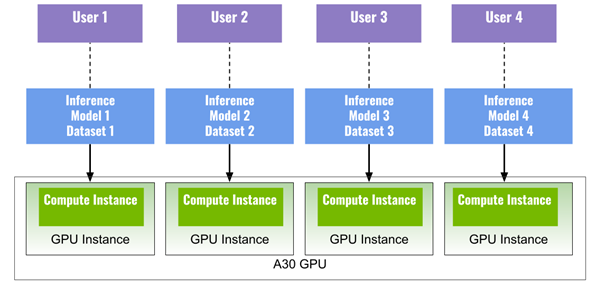
") No one likes standing around and waiting for the bus to arrive, especially when you need to be somewhere on time. Wouldn’t it be great if you could predict…
No one likes standing around and waiting for the bus to arrive, especially when you need to be somewhere on time. Wouldn’t it be great if you could predict…