
 Loss functions for training automatic speech recognition (ASR) models are not set in stone. The older rules of loss functions are not necessarily optimal….
Loss functions for training automatic speech recognition (ASR) models are not set in stone. The older rules of loss functions are not necessarily optimal. Consider connectionist temporal classification (CTC) and see how changing some of its rules enables you to reduce GPU memory, which is required for training and inference of CTC-based models and more.
Overview of connectionist temporal classification
If you are going to train an ASR model, whether it’s a convolutional or recurrent neural network, a transformer, or a combination, you are most likely training it with the CTC loss.
CTC is simple and convenient because it does not require per-frame information about “what sound is pronounced when” (so-called audio-text time alignment). In most cases, this knowledge is simply unavailable, as in a typical ASR dataset of audio with associated text with no time marks.
True time alignment is not always trivial. Suppose that most of the recording is without speech with only one short phrase at the end. CTC loss does not tell the model when exactly to emit a prediction. Instead, it allows for every possible alignment and just regulates the form of these alignments.
Here’s how exactly CTC manages all possible ways to align audio against text.
First, the target text is tokenized, that is, words are sliced into letters or word pieces. The number of the resulting units (whatever they are) should be less than the number of audio “timeframes”: segments of audio of length 0.01 to 0.08 seconds.
If there are fewer timeframes than units, then the algorithm fails. In this case, you should make your timeframes shorter. Otherwise, only RNN Transducer can save you. If the timeframes are as many as the units, then there can be only one alignment (a one-in-a-million case).
Most of the time, there are way more timeframes than units, so some of the frames are left without a unit. For such empty frames, CTC has a special unit. This unit tells you that the model has nothing to give you at this particular frame. This may be because there is no speech, or maybe the model is just too lazy to predict something meaningful here. The ability to predict nothing if the model doesn’t want to do that is provided by the most important rule of the CTC: the rule.
Other rules are related to unit continuation. Suppose that your unit is a vowel that lasts longer than one frame. On which of two frames should the model output the unit? CTC allows for the same unit emission on multiple consecutive frames. But then, the same consecutive units should be merged into one to convert the recognition results into a sequence of units that resembles text.
Now, what if your tokenized text itself contains the same repeated units like “ll” or “pp”? If left unprocessed, these units are merged into one even if they shouldn’t be. For this special case, CTC has a rule that if the target text has repeated units, then such units must be separated by during inference.
To sum up, in almost every frame, the model is allowed to emit the same unit from the previous frame, , or the next unit if it is different from the previous one. These rules are more sophisticated than the rule and they are not exactly necessary for CTC to work.
CTC implementation
Here’s how CTC loss can be represented. Like most loss functions in machine learning, it is usually represented as a dynamic algorithm that applies these rules to a training utterance or to the model’s softmax output.
In training, loss values and gradients are computed from conditional probabilities of all possible alignments by the Baum–Welch algorithm, applied to the CTC rules. The CTC implementations often have hundreds to thousands of lines of code and can be hard to modify.
Fortunately, there is another way to implement CTC. The weighted finite-state transducers (WFST) approach, apart from other application areas, allows the model to represent a dynamic algorithm as a set of graphs and associated graph operations. This approach enables you to decouple the CTC rules by applying them to specific audio and text and by calculating loss and gradients.
CTC WFST applications
With WFST, you can easily take the CTC rules and use them with different criteria, like maximum mutual information (MMI). These models usually have a lower word error rate (WER) than CTC models. MMI incorporates prior language information into the training process.
In contrast to CTC, MMI not only maximizes the probability of the most feasible path but also minimizes the probabilities of every other path. To do this, MMI has a so-called denominator graph, which can occupy a lot of GPU memory during training. Fortunately, some CTC rules can be modified to reduce denominator memory consumption without compromising speech recognition accuracy.
Also, a WFST representation of CTC rules, or a so-called topology, can be used to allow for WFST decoding of CTC models. To do that, you convert an N-gram language model to a WFST graph and compose it with the topology graph. The resulting decoding graph can be passed to, for example, the Riva CUDA WFST Decoder.
Decoding graphs can be large to the point that they may not fit in GPU memory. But with some CTC topology modifications, you can reduce decoding graph sizes for CTC.
CTC topologies
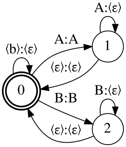
Figure 1 shows the CTC topology, Correct-CTC. This is a directed complete graph with self-loops, so for N units, including blank, there are N states and the square number of arcs.
Correct-CTC is the most commonly used CTC representation. Look at the typical sizes that this topology produces. For the LibriSpeech 4-gram word language model and 256 units of the model vocabulary, the decoding graph size is ~16Gb. Cold-start MMI training on a 32Gb GPU with the model vocabulary size 2048 is possible only with batch size 1.

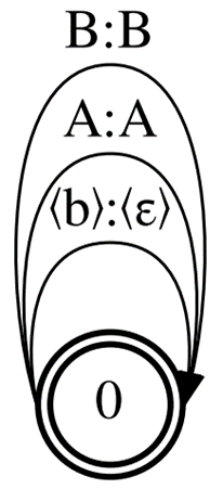
Reduce the memory consumption induced by Correct-CTC by dropping some of the CTC rules. First, drop the mandatory separation of repeated units with . Without this rule, you end up with the topology called Compact-CTC ( Figure 2). It has 3N – 2 arcs for N units.
Despite having pure 
Decoding graph sizes with Compact-CTC are a quarter smaller than with Correct-CTC. It also requires 2x less GPU memory for MMI training.
Now drop the same unit emission on multiple consecutive frames, leaving only the rule. This way, you end up with a topology with only one state and N arcs for N units.
This is the smallest possible CTC topology, so we call it Minimal-CTC (Figure 3). It requires even less GPU memory for MMI training (4x less compared to Correct-CTC), but the accuracy of an MMI-trained model with the Minimal-CTC topology will degrade compared to the baseline.
The smallest topology also produces the smallest decoding WFSTs with half the size of the baseline graph. Decoding graphs compiled with Minimal-CTC are incompatible with models built with Correct-CTC or Compact-CTC.
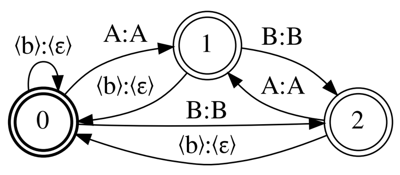
Finally, l come back to Correct-CTC but this time leave mandatory separation of repeated units and drop unit continuation. The topology called Selfless-CTC was designed to remedy the shortcomings of Minimal-CTC.
Figures 1 and 4 show that Correct-CTC and Selfless-CTC differ only in non- self-loops. These two topologies also give the same MMI model accuracy and an even better one if the model has a long context window. However, Selfless-CTC is also compatible with Minimal-CTC at decoding. You get the 2x graph size reduction from Minimal-CTC by the cost of only 0.2% higher WER.
Conclusion
There are several tips for better performance:
- Use Compact-CTC instead of Correct-CTC for decoding graph construction and MMI training.
- For the best decoding graph size reduction, train your models with Selfless-CTC and decode with Minimal-CTC.
- Loss functions are not set in stone: Experiment with your own WFST representations of existing loss functions and create new ones. It’s fun!
For more information, see CTC Variations Through New WFST Topologies or view the INTERSPEECH session.
Other useful resources:
- MMI training with NVIDIA NeMo
- A fast standalone WFST decoder that supports CTC models with different topologies
- Differentiable WFSTs for making topologies and more: