Boosting Dynamic Programming Performance Using NVIDIA Hopper GPU DPX Instructions

Dynamic programming (DP) is a well-known algorithmic technique and a mathematical optimization that has been used for several decades to solve groundbreaking…

Dynamic programming (DP) is a well-known algorithmic technique and a mathematical optimization that has been used for several decades to solve groundbreaking problems in computer science.

An example DP use case is route optimization with hundreds or thousands of constraints or weights using the Floyd-Warshall all-pair shortest paths algorithm. Another use case is the alignment of reads for genome sequence alignment using the Needleman-Wunsch or Smith-Waterman algorithms.

NVIDIA Hopper GPU Dynamic Programming X (DPX) instructions accelerate a large class of dynamic programming algorithms used in areas such as genomics, proteomics, and robot path planning. Accelerating these dynamic programming algorithms can help researchers, scientists, and practitioners glean insights much faster about the underlying DNA or protein structures and several other areas.

What is dynamic programming?

DP techniques initially involve expressing the algorithm recursively, where the larger problem is broken down into subproblems that are easier to solve.

A common computational optimization used in DP is to save the results of the subproblems and use them in subsequent steps of the problem, instead of recomputing the solution each time. This step is called memoization. Memoization facilitates avoiding the recursion steps and instead enables using an iterative, look-up, table–based formulation. The previously computed results are stored in the look-up table.

One of the key observations in many DP problems is that the solution to a larger problem often involves computing the minimum or maximum of the previously computed solutions. The larger problem’s solution is within a delta of that min-max of previous solutions.

DP techniques, in general, achieve the same results as brute force algorithms, but with dramatic reductions in the computational requirements and execution times.

DP example: Accelerating the Smith-Waterman algorithm

NVIDIA Clara Parabricks is a GPU-accelerated genomic analysis suite of tools that heavily uses the Smith-Waterman algorithm and runs on NVIDIA GPUs: A100, V100, A40, A30, A10, A6000, T4, and soon the newest H100.

Genome sequencing has fundamental applications with universal benefits, with examples that include personalized medicine or tracking disease spread. Every cell in living organisms encodes genetic information using a sequence of four nucleotides in DNA (or bases). The nucleotides are adenine, cytosine, guanine, and thymine, represented by A, C, T, and G.

Simple organisms like viruses have a sequence of 10–100K bases while human DNA consists of about three billion base pairs. There are instruments (chemical– or electrical-signal–based) that sequence the bases of short segments of genetic material, called reads. These reads are typically 100–100K bases long, depending on the sequencer technology used for gathering the reads.

A critical computational step in genome sequence analysis is to align the reads to find the best match among a pair of reads. These reads can be 100-400 base pairs long in second-generation sequencers, and up to 100K bases long in third-generation sequencers. Aligning reads is a computational step that is repeated tens or hundreds of millions of times.

There are challenges in finding the best match that include the following:

Naturally occurring variations in genomes that give organisms within a species their specific traits
Errors in the reads themselves resulting from the sequencing instrument or underlying chemical processes

The best match between a pair of reads is equivalent to an approximate string match between a pair of strings with steps that reward matches and penalize differences. The differences between the reads could be mismatches, insertions, or deletions.

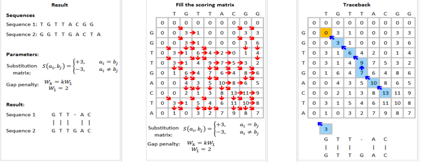
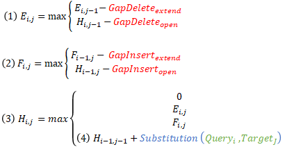
The Smith-Waterman algorithm proceeds to find the best match between a pair of sequences TGTTACGG and GGTTGACTA. — *Figure 1. Smith-Waterman scoring matrix and traceback for a pair of sequences (*Source: Wikipedia)

Figure 1 shows that the Smith-Waterman step in genomic sequencing aims to find the best match between the read sequences TGTTACGG and GGTTGACTA. The resulting best match is shown to be GTT-AC (from sequence 1, the “-” representing a deletion) with GTTGAC (from sequence 2). The scoring scheme in each step rewards matches (+3), penalizes mismatches (-3), and penalizes insertions and deletions (see the gap penalty formula in Figure 1).

This is an example formulation of the Smith-Waterman algorithm. Implementers of the Smith-Waterman algorithm are allowed to customize the rewards and penalties.

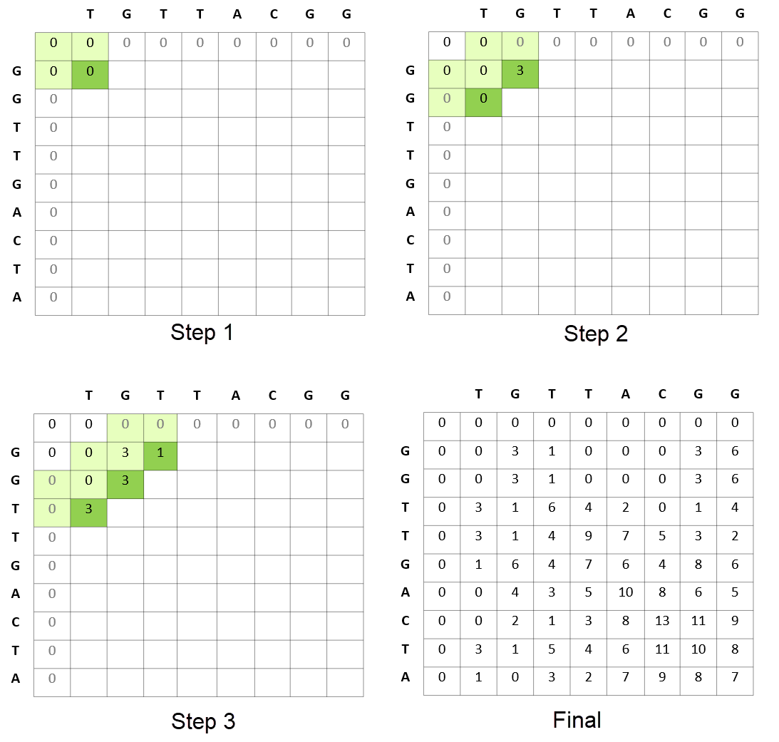
While computing the best match between TGTTACGG and GGTTGACTA, the Smith-Waterman algorithm also computes the best matches for all prefixes of TGTTACGG with all prefixes of GGTTGACTA. It proceeds from the start of these sequences and uses the results of the smaller prefixes to feed into the problem of finding the solution for the larger prefixes.

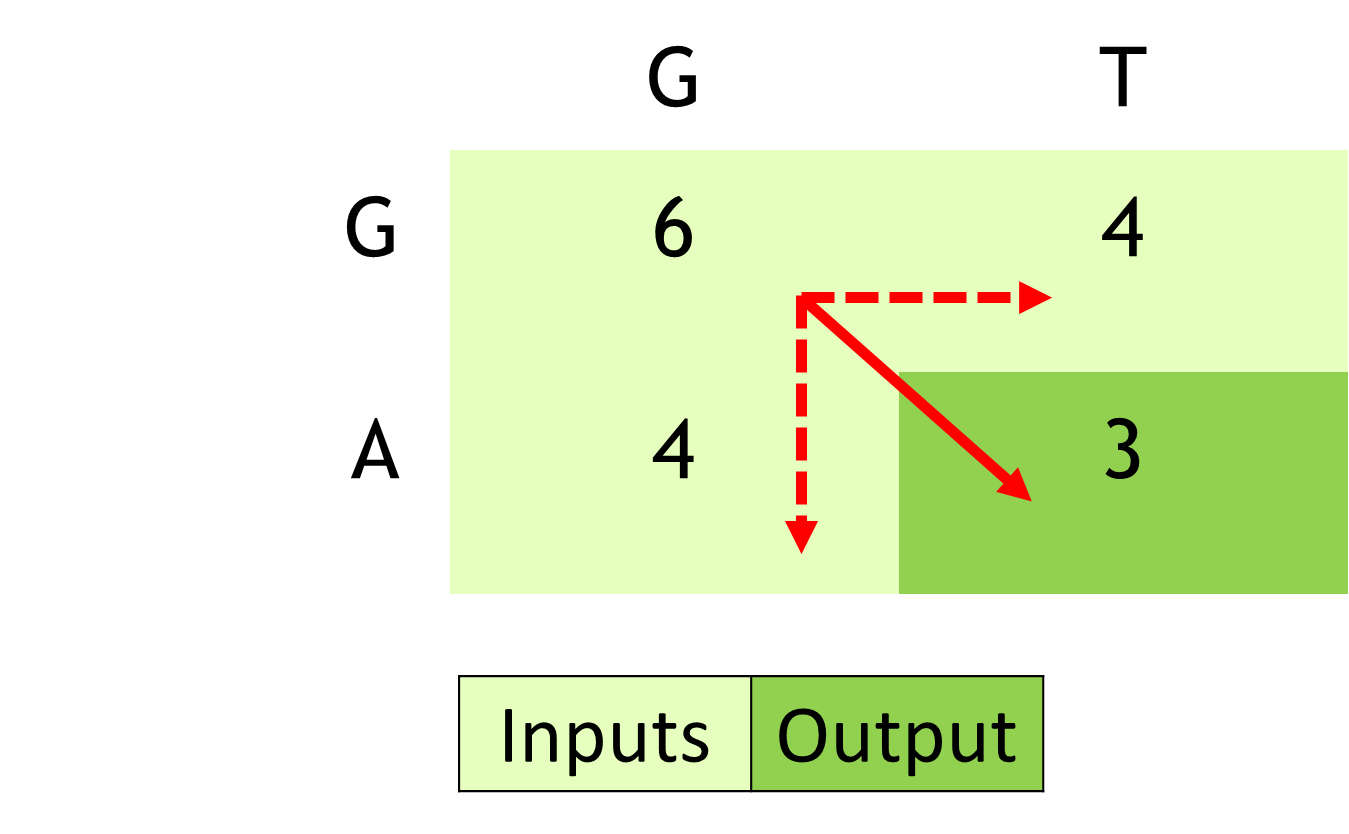
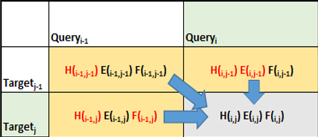
Diagram shows a simplified cell calculation step between GA and GT. Only the cell entry for A versus T has to be calculated. This is a mismatch. Take the maximum score after accounting for substitution and gap penalties. — *Figure 2. A simplified cell calculation step in the Smith-Waterman algorithm*

Figure 3 shows how the algorithm proceeds in terms of calculating the scores of matrices for matching a sequence of reads. This comparative matching is the computationally expensive step of the Smith-Waterman algorithm.

This is just one of the formulations of how the Smith-Waterman algorithm proceeds. Different formulations can result in the algorithm proceeding row-wise or column-wise as examples.

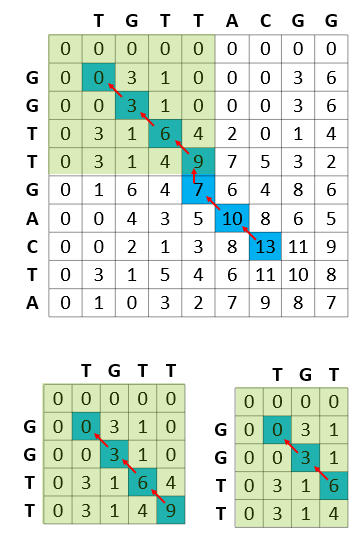
Each cell calculation requires the cell to the top, left, and top-left to be available. This diagram shows a formulation of Smith-Waterman that proceeds diagonally, starting from the top-left corner of the scoring matrix. — *Figure 3. Example steps of the Smith-Waterman algorithm*

After the score matrix is computed, the next step involves backtracking from the highest score to the origin of each of these scores. This is a computationally light step given that each cell maintains how it got its score (the source cell for score calculation).

If each cell keeps a tab of where the score was derived from (top, left, top-left), tracking back the score to a zero will show the best match(es) between the sequences. — *Figure 4. Backtracking from the highest score in the Smith-Waterman algorithm*

Figure 5 shows the computational efficiency of the Smith-Waterman calculations, where each of the subproblems solved by the algorithm is stored in the result matrix and never recomputed.

For example, in the process of calculating the best match of GGTTGACTA and TGTTACGG, the Smith-Waterman algorithm reuses the best match between GGTT (prefix of GGTTGACTA) and TGTT (prefix of TGTTACGG). In turn, while calculating the best match of GGTT and TGTT, the best match of all prefixes of these strings are calculated and reused (for example, best match of GGTT and TGT).

The best match of GGTT with TGTT also calculates the best match of GGTT with TGT. In fact, the best match with every prefix of TGTTACGG with every prefix of GGTTGACTA is calculated in the scoring matrix. — *Figure 5. Subproblems solved by the Smith-Waterman algorithm*

Leveraging DPX instructions for better performance

The inner loop in a real Smith-Waterman implementation involves the following for each cell:

Updating deletion penalties
Updating insertion penalties
Updating the score based on the updated insertion and deletion penalties.

Equations for the insertion and deletion penalties.

Practical implementations of Smith-Waterman must keep tabs of the insertion and deletion penalties in addition to the scores. — *Figure 6. Updating insertion penalty, deletion penalties, and scores in a Smith-Waterman implementation step*

The NVIDIA Hopper Architecture math API provides dramatic acceleration for such calculations. The APIs expose the acceleration provided by NVIDIA Hopper Streaming Multiprocessor for additions followed by minimum or maximum as a fused operation (for example, __viaddmin_s16x2_relu, an intrinsic that performs per-halfword 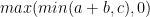$max(min(a + b, c), 0)$ ).

Another example of an API that is extensively leveraged by Smith-Waterman software is a three-way min or max followed by a clamp to zero ( for example, __vimax3_s16x2_relu, an intrinsic that performs per-halfword $max(max(max(a, b), c), 0)$ ).

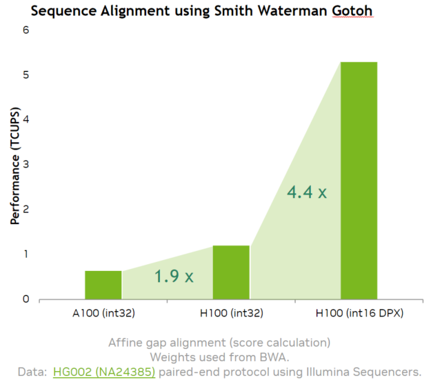
Our implementation of the Smith-Waterman algorithm using the NVIDIA Hopper DPX instruction math APIs provides a 7.8x speedup over A100.

NVIDIA Hopper DPX instructions enable over a 7x speedup for the Smith-Waterman score matrix calculations. — *Figure 7. Smith-Waterman calculations speedup using DPX instructions in H100*

Needleman-Wunsch and partial order alignment

In the same way that Smith-Waterman algorithms use DPX instructions, there is a large family of alignment algorithms that essentially use the same principles.

Examples include the Needleman-Wunsch algorithm in which the basic flow of the algorithm resembles the Smith-Waterman closely. However, the initialization, insertion, and gap penalties are calculated differently between these two approaches.

Algorithms like Partial Order Alignment make dense use of cell calculations that closely resemble Smith-Waterman cell calculations in their inner loop.

All-pair shortest paths

Robotic path planning with thousands or tens of thousands of objects is a common problem in warehouses where the environment is dynamic with many moving objects. These scenarios can involve dynamic replanning every few milliseconds.

The inner loop of most all-pair shortest paths algorithms is as shown using the following Floyd-Warshall algorithm example. The pseudocode shows how the all-pair shortest paths algorithm has an inner loop that updates the min distance between each vertex pair. The most-dense operation is essentially an add followed by a min operation.

initialize(dist); # initialize nearest neighbors to actual distance, all others = infinity 
for k in range(V): #order of visiting k values not important, must visit each value

	# pick all vertices as source in parallel
	Parallel for_each i in range(V):

		# Pick all vertices as destinations for the
		# above picked source
		Parallel for_each j in range(V):

			# If vertex k is on the shortest path from
			# i to j, then update the value of dist[i][j]
			dist[i][j] = min (dist[i][j], dist[i][j] + dist[k][j])

			# dist[i][j] calculation can be parallel within each k
			# All dist[i][j] for a single ‘k’ must be computed 
                        # before moving to the next ‘k’
		Synchronize

The speedup offered by DPX instructions makes it possible to dramatically scale the number of objects analyzed or have the re-optimization done in real time with fewer GPUs and optimal results.

Accelerate dynamic programming algorithms with DPX instructions

Using NVIDIA Hopper DPX instructions demonstrated speedups of up to 7.8x on the A100 GPU for Smith-Waterman, which is key in many genomic sequence alignment and variant calling applications. The exposure in math APIs, available in CUDA 12, enables the configurable implementation of the Smith-Waterman algorithm to suit different user needs, as well as algorithms like Needleman-Wunsch.

DPX instructions accelerate a large class of dynamic programming algorithms such as DNA or protein sequencing, and robot path planning. Most importantly, these algorithms can lead to dramatic speed-ups in disease diagnosis, drug discoveries, and robot autonomy, making our everyday lives better.

Acknowledgments

We’d like to thank Bill Dally, Alejandro Cachon, Mehrzad Samadi, Shirish Gadre, Daniel Stiffler, Rob Van der Wijngaart, Joseph Sullivan, Nikita Astafev, Seamus O’Boyle, and many others across NVIDIA.