
 Nowadays, a huge number of implementations of state-of-the-art (SOTA) models and modeling solutions are present for different frameworks like TensorFlow, ONNX,…
Nowadays, a huge number of implementations of state-of-the-art (SOTA) models and modeling solutions are present for different frameworks like TensorFlow, ONNX, PyTorch, Keras, MXNet, and so on. These models can be used for out-of-the-box inference if you are interested in categories already in the datasets, or they can be embedded to custom business scenarios with minor fine-tuning.
This post gives you an overview of prevalent DL model categories and walks you through the end-to-end examples of deploying these models using NVIDIA Triton Inference Server. The client applications can be used as it is or can be modified according to the use case scenarios. I walk you through the deployment of image classification, object detection, and image segmentation public models using Triton Inference Server. The steps outlined in this post can also be applied to other open-source models with minor changes.
Deep learning inference challenges
Recent years have seen remarkable advancements in deep learning (DL). By resolving numerous complex and intricate problems that have hampered the AI community for years, it has completely revolutionized the future of AI. It is currently being used with rapidly growing applications in different industries, ranging from healthcare and aerospace engineering to autonomous driving and user authentications.
Deep learning, however, has various challenges when it comes to inference:
- Support of multiple frameworks
- Ease of use
- Cost of deployment
Support of multiple frameworks
The first key challenge is around supporting multiple different types of model frameworks.
Developers and data scientists today are using various frameworks for their production models. For instance, there can be difficulties modifying the system for testing and deployment if a machine learning project is written in Keras, but a team member has more experience with TensorFlow.
Also, converting the models can be expensive and complicated, especially if new data is required for their training. They must have a server application to support each of those models.
Ease of use
The next key challenge is to have a serving application that can support different inference queries and use cases.
In some applications, you’re focused on real-time online inferencing where the priority is to minimize latency as much as possible. On the other hand, there might be use cases that require you to do offline batch inferencing where you’re focused on maximizing throughput.
It’s essential to have solutions that can support each type of query and use case and optimize for them.
Cost of deployment
The next challenge is managing the cost of deployment and lowering the cost of inference.
A key part of this is having one serving application that can support running on a mixed infrastructure. You might create a separate serving solution for running on CPU, another one for GPU, and a different one for deploying on the cloud in the data center and edge. That’s going to skyrocket costs and lead to a nonscalable implementation.
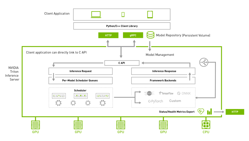
Triton Inference Server
Triton Inference Server is an open-source server inference application allowing inference on both CPU and GPU in different environments. It supports various backends, including TensorRT, PyTorch, TensorFlow, ONNX, and Python. To have maximum hardware utilization, NVIDIA Triton allows concurrent execution of different models. Further dynamic batching allows grouping together inference queries to maximize the throughput for different types of queries. For more information, see NVIDIA Triton Inference Server.
Quickstart with NVIDIA Triton
The easiest way to install and run NVIDIA Triton is to use the pre-built Docker image available from NGC.
Server: Pull the Docker image
Pull the image using the following command:
$ docker pull nvcr.io/nvidia/tritonserver:-py3NVIDIA Triton is optimized to provide the best inferencing performance by using GPUs, but it can also work on CPU-only systems. In both cases, you can use the same Docker image.
Use the following command to run NVIDIA Triton with the example model repository that you just created:
docker run --gpus=1 --rm --net=host -v /path/to/the/repo/server/models:/models nvcr.io/nvidia/tritonserver:-py3 tritonserver --model-repository=/models --exit-on-error=false --repository-poll-secs=10 --model-control-mode="poll"Client: Get the client libraries
Use docker pull to get the client libraries.
$ docker pull nvcr.io/nvidia/tritonserver:-py3-sdkIn this command, is the version to pull. Run the client image.
To start the client, run the following command:
$ docker run -it --rm --net=host /path/to/the/repo/client/:/python_examples nvcr.io/nvidia/tritonserver:-py3-sdkEnd-to-end model deployment
The NVIDIA Triton project provides several client libraries in C++ and Python to simplify communication. These APIs make communicating with NVIDIA Triton easy. With the help of these APIs, the client applications process the input and communicate with NVIDIA Triton to perform inferencing.

In general, the interaction of client applications with NVIDIA Triton can be summarized as follows:
- Input
- Preprocess
- Inference
- Postprocess
- Output
Input: Depending upon the application type, one or more inputs are read to be inferred by the neural network.
Preprocess: Preprocessing data is a common first step in the deep learning workflow to prepare raw data in a format the network can accept, For example, image resizing, normalization, or noise removal from input data.
Inference: For the inference part, a client initially serializes the inference request into a message and sends it to Triton Inference Server. The message travels over the network from the client to the server and gets deserialized. The request is placed on the queue. The request is removed from the queue and computed. The completed request is serialized in a message and sent back to the client. The message travels over the network from the server to the client. The message arrives at the client and is deserialized.
Postprocess: When the message arrives at the client application, it is processed as a completed inference request. Depending upon the network type and application use case, post-processing is applied. For example, in object detection, postprocessing involves suppressing the superfluous boxes, aiding in selecting the best possible boxes, and mapping them back to the input image.
Output: After inference and processing, depending upon the application, the output can be stored, displayed, or passed to the network.
Image classification
Image classification is the task of comprehending an entire image and specifying a specific label for the image. Typically in image classification, a single object is present in the image, which is analyzed and comprehended. For more information, see image classification.
Server: Download the model
Download the ResNet-18 image classification model from the ONNX model zoo:
$ cd /path/to/the/repo/server/models/classification/1
$ wget https://github.com/onnx/models/raw/main/vision/classification/resnet/model/resnet18-v1-7.onnx && mv resnet18-v1-7.onnx model.onnx
The following code example shows the model configuration file:
name: "classification"
platform: "onnxruntime_onnx"
max_batch_size : 1
input [
  {
    name: "data"
    data_type: TYPE_FP32
    format: FORMAT_NCHW
    dims: [ 3, 224, 224 ]
    reshape { shape: [ 3, 224, 224 ] }
  }
]
output [
  {
    name: "resnetv15_dense0_fwd"
    data_type: TYPE_FP32
    dims: [  1000 ]
    reshape { shape: [1000] }
    label_filename: "labels.txt"
  }
]
Name, platform, and backend
The name property is optional. If the name of the model is not specified in the configuration, it is assumed to be the same as the model repository directory containing the model. The model is executed by the NVIDIA Triton backend, which is simply a wrapper around the DL frameworks like TensorFlow, PyTorch, TensorRT, and so on. For more information, see backend.
Maximum batch size
The maximum batch size that a model can support is indicated by the max_batch_size property. Zero size shows that bathing is not supported. For more information, see batch size.
Inputs and outputs
For each model, the expected input, output, and data types must be specified in the model configuration file. Based on the input and output tensors, different data types are allowed. For more information, see Datatypes.
The image classification model accepts a single input, and after the inference returns a single output.
In a separate console, launch the image_client example from the NGC NVIDIA Triton container.
Client: Run the image classification client
To run the image classification client, use the following command:
$ python3 /python_examples/examples/classification/classification.py -m classification -s INCEPTION /python_examples/examples/images/tabby.jpgFirst, inputs are preprocessed according to the model. For this model, inception scaling is applied, which scales the input as follows:
if scaling == 'INCEPTION':
    scaled = (typed / 127.5) - 1
The inference request is sent to NVIDIA Triton, and the responses are appended:
responses.append(
    triton_client.infer(FLAGS.model_name,
                        inputs,
                        request_id=str(sent_count),
                        model_version=FLAGS.model_version,
                        outputs=outputs))
Finally, the responses obtained from the server are post-processed.
postprocess(response, output_name, FLAGS.batch_size, supports_batching)For the classification case, the model returns a single classification output that comprehends the input image. The class is decoded and printed in the console.
for results in output_array:
    if not supports_batching:
        results = [results]
    for result in results:
        if output_array.dtype.type == np.object_:
            cls = "".join(chr(x) for x in result).split(':')
        else:
            cls = result.split(':')
        print("    {} ({}) = {}".format(cls[0], cls[1], cls[2]))
For more information, see classification.py.
Figure 4 shows the sample output.

Object detection
The process of finding instances of objects of a particular class within an image is known as object detection. The problem of object detection combines classification with localization. It also examines more plausible scenarios in which an image might contain several objects. For more information, see object detection.
Server: Download the model
Download the faster_rcnn_inception_v2_coco object detection model:
$ cd /path/to/the/repo/server/models/detection/1
$ wget http://download.tensorflow.org/models/object_detection/faster_rcnn_inception_v2_coco_2018_01_28.tar.gz && tar xvf faster_rcnn_inception_v2_coco_2018_01_28.tar.gz && cp faster_rcnn_inception_v2_coco_2018_01_28/frozen_inference_graph.pb ./model.graphdef &&  rm -r faster_rcnn_inception_v2_coco_2018_01_28 faster_rcnn_inception_v2_coco_2018_01_28.tar.gz
The following code example shows the model configuration file for the object detection model:
name: "detection"
platform: "tensorflow_graphdef"
max_batch_size: 1
input [
  {
    name: "image_tensor"
    data_type: TYPE_UINT8
    format: FORMAT_NHWC
    dims: [ 600, 1024, 3 ]
  }
]
output [
  {
    name: "detection_boxes"
    data_type: TYPE_FP32
    dims: [ 100, 4]
    reshape { shape: [100,4] }
  },
  {
    name: "detection_classes"
    data_type: TYPE_FP32
    dims: [ 100 ]
    reshape { shape: [ 1, 100 ] }
  },
  {
    name: "detection_scores"
    data_type: TYPE_FP32
    dims: [ 100 ]

  },
  {
    name: "num_detections"
    data_type: TYPE_FP32
    dims: [ 1 ]
    reshape { shape: [] }
  }
]
The detection model accepts a single image as an input and returns four different outputs.
Client: Run the object detection client
To run the object detection client, use the following command:
$ python3 /python_examples/examples/detection/detection.py -m detection /python_examples/examples/images/car.jpgThe object detection model returns four different outputs, which are decoded in the post-processing step:
detection_boxes = results.as_numpy(output_name[0].name)
detection_classes = results.as_numpy(output_name[1].name)
detection_scores = results.as_numpy(output_name[2].name)
num_detections = results.as_numpy(output_name[3].name)
At the end, the bounding boxes are drawn on the input as follows:
for idx, detection_box in enumerate(detection_boxes[0,0:int(num_detections),:]):
    y_min=int(detection_box[0]*w)
    x_min=int(detection_box[1]*h)
    y_max=int(detection_box[2]*w)
    x_max=int(detection_box[3]*h)
    start_point = (x_min,y_min)
    end_point = (x_max,y_max)
    shape = (start_point, end_point)
    draw.rectangle(shape, outline ="red")
    draw.text((int((x_min+x_max)/2),y_min), "class-"+str(int(detection_classes[0,idx])), fill=(0,0,0))
For more information, see detection.py.
Figure 5 shows the sample output.
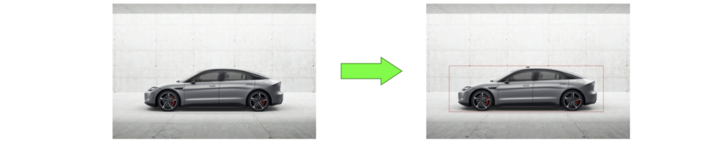
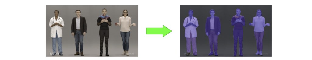
Image segmentation
The process of clustering parts of an image that correspond to the same object class is known as image segmentation. Image segmentation entails splitting images or video frames into multiple objects or segments. For more information, see image segmentation.
Server: Download the model
To download the model, use the following commands:
$ cd /path/to/the/repo/server/models/segmentation/1
$ wget https://github.com/onnx/models/raw/main/vision/object_detection_segmentation/fcn/model/fcn-resnet50-11.onnx &&  mv fcn-resnet50-11.onnx model.onnx
The following code example shows the model configuration file for the image segmentation model:
name: "segmentation"
platform: "onnxruntime_onnx"
max_batch_size : 0
input [
  {
    name: "input"
    data_type: TYPE_FP32
    format: FORMAT_NCHW
    dims: [  3, -1, -1 ]
    reshape { shape: [ 1, 3, -1, -1 ] }
  }
]
output [
    {
    name: "out"
    data_type: TYPE_FP32
    dims: [  -1, 21, -1, -1 ]
  }
]
Client: Run the image classification client
To run the image classification client, run the following commands:
$ pip install opencv-python
$ python3 /python_examples/examples/segmentation/segmentation.py -m segmentation -s INCEPTION /python_examples/examples/images/people.jpg
The segmentation model accepts a single input and returns a single output. After inferencing, the model returns the output based on which segmented and blended images are generated.
# generate segmented image
result_img = colorize(raw_labels)
# generate blended image
blended_img = cv2.addWeighted(image[:, :, ::-1], 0.5, result_img, 0.5, 0)
For more information, see the segmentation.py file.
Figure 6 shows the sample output.
Resources
Try Triton Inference Server today on GPU, CPU, or both. The NVIDIA Triton Inference Server container can be downloaded from NGC, and its source code is available on the /triton-inference-server GitHub repo.
- For documentation, see Triton Inference Server on GitHub.
- If you’re looking for a hands-on skills lab, see Efficient Cloud-based Deployment of Deep Learning Models using Triton Inference Server and TensorRT.
- For scalable model deployment with NVIDIA Triton Inference Server, see Fast and Scalable AI Model Deployment with NVIDIA Triton Inference Server.
- See Simplifying AI Inference in Production with NVIDIA Triton.
- If you’re interested in inferencing of large models, see Accelerated Inference for Large Transformer Models Using NVIDIA Triton Inference Server.
- For a copy of the code used in this post, see /arslana/triton_blog_1 on Gitlab.
 Examples of what a smart city is can be found in metro IoT deployments from Singapore to Seat Pleasant, Maryland.
 Learn how to write simple, portable, parallel-first GPU-accelerated applications using only C++ standard language features in this self-paced course from the…
 From taking your order and serving you food in a restaurant to playing poker with you, service robots are becoming increasingly prevalent. Globally, you can…
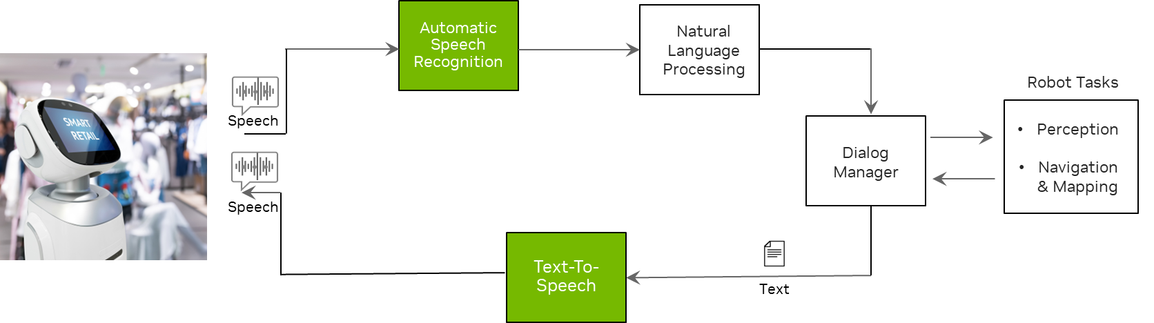
 Speech is one of the primary means to communicate with an AI-powered application. From virtual assistants to digital avatars, voice-based interfaces are…
 Loading and preprocessing data for running machine learning models at scale often requires seamlessly stitching the data processing framework and inference…
 A pretrained AI model is a deep learning model that’s trained on large datasets to accomplish a specific task, and it can be used as is or customized to suit…