The human hand is one of the most remarkable outcomes of millions of years of evolution. The ability to pick up all sorts of objects and use them as tools is a…
The human hand is one of the most remarkable outcomes of millions of years of evolution. The ability to pick up all sorts of objects and use them as tools is a crucial differentiator enabling us to shape our world.
For robots to work in the everyday human world, the ability to deftly interact with our tools and the environment around them is critical. Without that capability, they will continue to be useful only in specialized domains such as factories or warehouses.
While it has been possible to teach robots with legs how to walk for some time, robots with hands have generally proven to be much more tricky to control. A hand with fingers has more joints that must move in specific coordinated ways to accomplish a given task. Traditional robotics control methods with precise grasps and motions are incapable of the kind of generalized fine motor control skills that humans take for granted.
One approach to these problems has been the application of deep reinforcement learning (deep RL) techniques that train a neural network to control the robot’s joints. With deep RL, a robot learns from trial and error and is rewarded for the successful completion of the assigned task. Unfortunately, this technique can require millions or even billions of samples to learn from, making it almost impossible to apply directly to real robots.
Applying simulation
Enter the NVIDIA Isaac robotics simulator, which enables robots to be trained inside a simulated universe that can run more than 10,000x faster than the real world and yet obeys the laws of physics.
Using NVIDIA Isaac Gym, an RL training robotics simulator, NVIDIA researchers on the DeXtreme project taught this robot hand how to manipulate a cube to match a provided target position and orientation or pose. The neural network brain learned to do this entirely in simulation before being transplanted to control a robot in the real world.
Similar work has only been shown one time before, by researchers at OpenAI. Their work required a far more sophisticated and expensive robot hand, a cube tricked out with precise motion control sensors, and a supercomputing cluster of hundreds of computers to train.
Democratizing dexterity
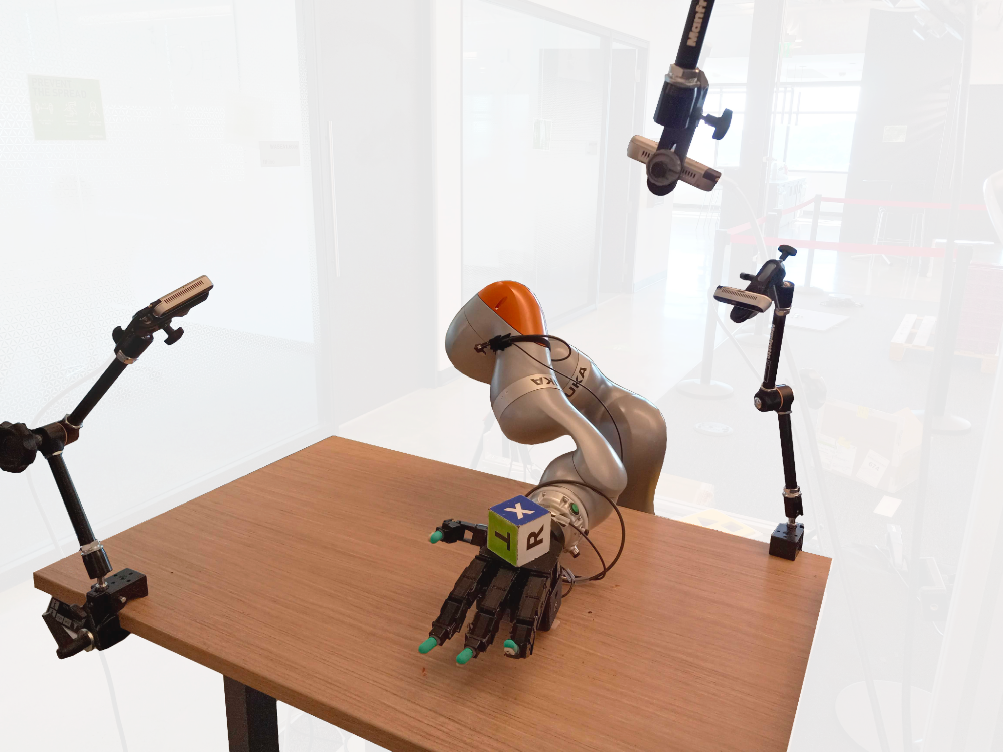
The hardware used by the DeXtreme project was chosen to be as simple and inexpensive as possible to enable researchers worldwide to replicate our experiments.
The robot itself is an Allegro Hand, which costs as little as 1/10th the cost of some alternatives, has four fingers instead of five, and has no moving wrist. We can use three off-the-shelf RGB cameras to track the 3D cube with vision, which can be repositioned easily as needed without requiring special hardware. The cube is 3D-printed with stickers affixed to each face.
DeXtreme is trained using Isaac Gym, which provides an end-to-end GPU-accelerated simulation environment for reinforcement learning. NVIDIA PhysX simulates the world on the GPU, and results stay in GPU memory during the training of the deep learning control policy network.
As a result, training can happen on a single Omniverse OVX server. Training a good policy takes about 32 hours on this system, equivalent to 42 years of a single robot’s experience in the real world.
Not needing a separate CPU cluster for simulation means a 10–200x reduction in computing costs for training at current cloud rental rates. Because we can use Isaac Gym to train the model, training time and cost can be dramatically reduced.
Perception and synthetic data
For the robot to know the current position and orientation of the cube that it’s holding, it needs a perception system. To keep costs low and leave open the potential for manipulation of other objects in the future, DeXtreme uses three off-the-shelf cameras and another neural network that can interpret the cube pose.
This network is trained using about 5 million frames of synthetic data generated using Omniverse Replicator and no real images whatsoever. The network learns how to perform the task under challenging circumstances in the real world. To make the training more robust, we use a technique called domain randomization to change lighting and camera positions, plus data augmentation to apply random crops, rotation, and backgrounds.
The DeXtreme pose estimation system is reliable and can perceive accurate poses even when the object in question is partly occluded from view, or when the image has significant motion blur.
Real robots are still challenging
One of the key reasons to use simulations is that training robots directly in the real world are riddled with various challenges. For example, robot hardware is prone to breaking after excessive usage. Experiment iteration cycles and turnaround time can also be slow.
During our experiments, we often found ourselves repairing the hand after prolonged usage, for example, tightening the loose screws, replacing the ribbon cables, and resting the hand to cool down after running 10-15 trials. Simulations enabled us to sidestep many of these issues by training on a robot that doesn’t wear out but also provides the large diversity of data needed to learn challenging tasks. At the same time, because simulations can run much faster than in real time, the iteration cycle is massively improved.
When training in simulation, the most significant challenge is bridging the gaps between the simulations and the real world. To address this, DeXtreme uses domain randomization of the physics properties set in the simulator: changing object masses, friction levels, and other attributes at scale across over a hundred thousand simulated environments at one time.
One interesting upshot of these randomizations is that we train the AI with all kinds of unusual combinations of scenarios, which translates to robustness when performing the task in the real world. For instance, most of our experiments on the real robot took place with a slightly malfunctioning thumb due to a loose connection on the circuit board. We were positively surprised that the policies transferred from simulation to the real world reliably, regardless.
Video 5. After over 32 hours of training, the DeXtreme robot was capable of repeated success at the task of rotating a cube to match a specific target
Sim-to-real
Future breakthroughs in robotic manipulation will enable a new wave of robotics applications beyond traditional industrial uses.
At the heart of the DeXtreme project is the message that simulation can be an incredibly effective tool for training complex robotic systems. This is true even for the systems that must handle environments with objects in continual contact with the robot. We hope that by demonstrating this using relatively low-cost hardware, we can inspire others to use our simulation tools and build on this work.
For more information, see DeXtreme: Transfer of Agile In-hand Manipulation from Simulation to Reality and visit DeXtreme.
For a further dive into simulators and how they can affect your projects, see How GPUs Can Democratize Deep Reinforcement Learning for Robotics Development. You can also download the latest version of NVIDIA Omniverse Isaac Sim and learn about training your own reinforcement learning policies.


 NVIDIA Modulus is now available on NVIDIA LaunchPad. Sign-up for a free, hands-on lab that will teach you how to develop physics-informed machine-learning…
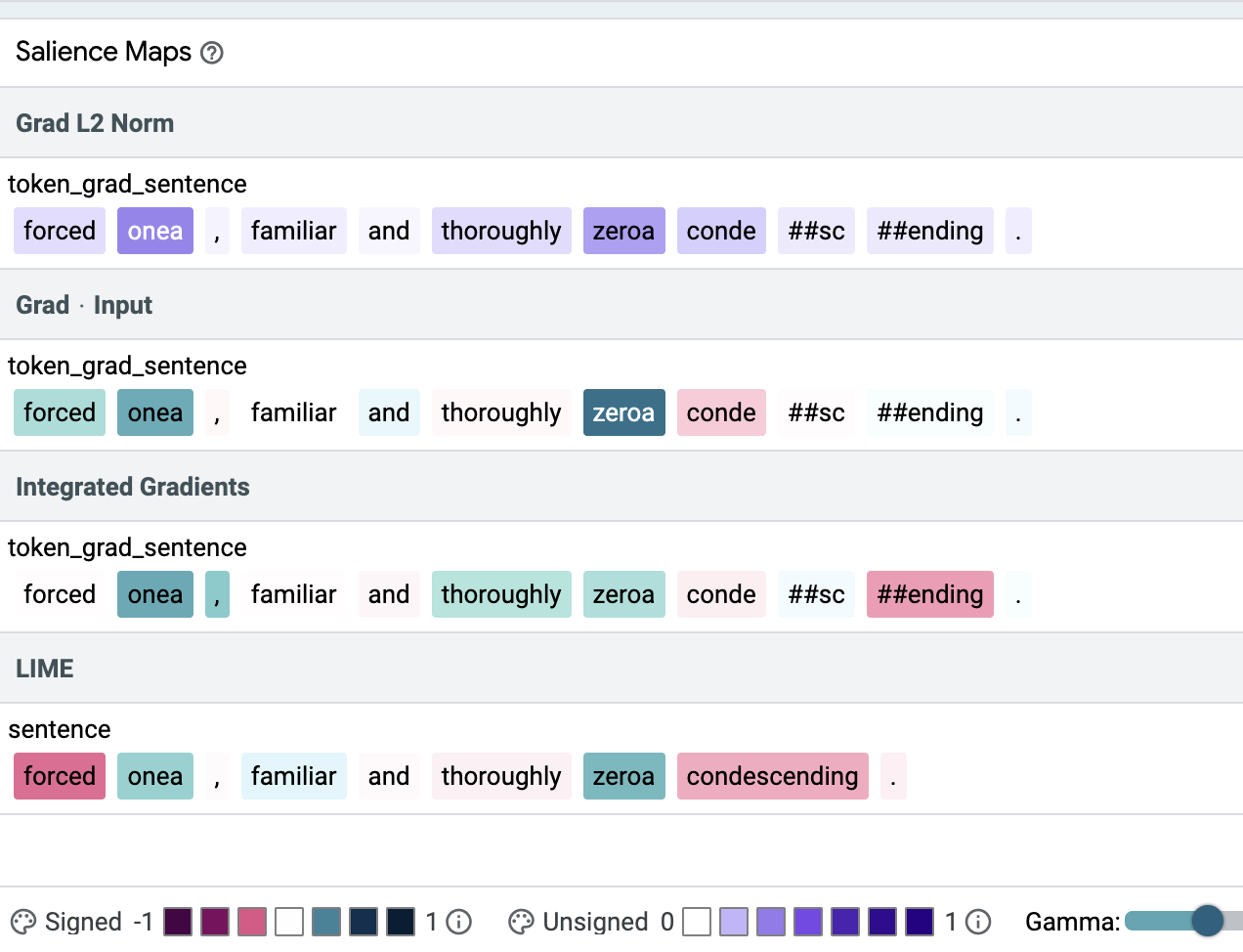
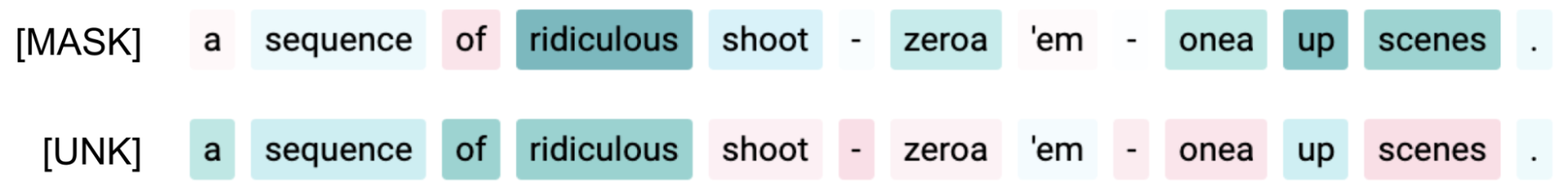
 HDBSCAN is a state-of-the-art, density-based clustering algorithm that has become popular in domains as varied as topic modeling, genomics, and geospatial…
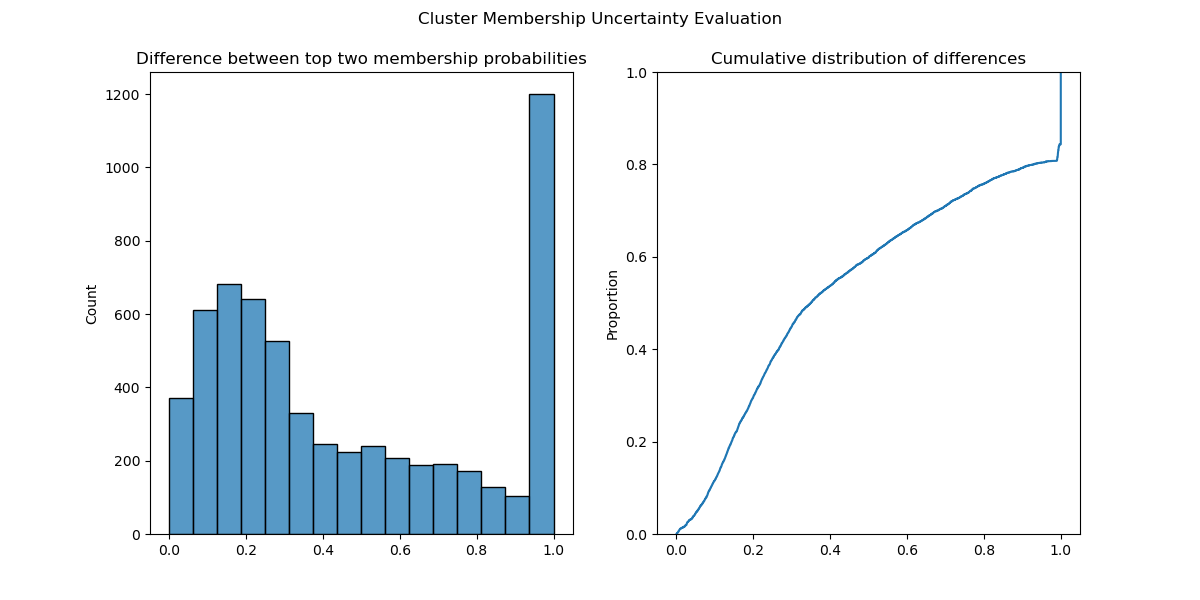
 X-ray-powered research is aiming to target sneaky hazardous materials making their way through airport security. The study, recently published in Scientific…
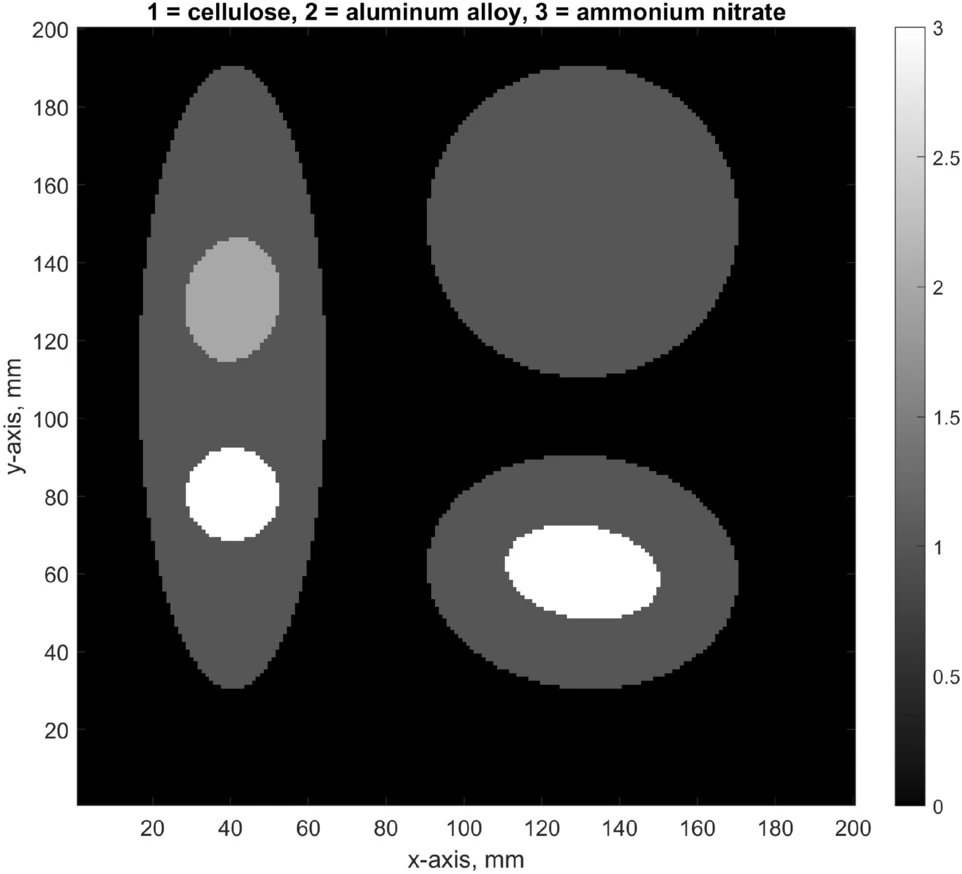
 The NVIDIA Optical Flow SDK 4.0 is now available, enabling you to fully harness the new NVIDIA Optical Flow Accelerator on the NVIDIA Ada architecture with…
 The NVIDIA Base Command Platform enables an intuitive, fully featured development experience for AI applications. It was built to serve the needs of…
 Real-time natural language understanding will transform how we interact with intelligent machines and applications.
 The role of artificial intelligence (AI) in boosting performance and energy efficiency in cellular network operations is rapidly becoming clear. This is…