
Month: June 2023
Categories
Optimizing Memory with NVIDIA Nsight Systems
 NVIDIA Nsight Systems is a comprehensive tool for tracking application performance across CPU and GPU resources. It helps ensure that hardware is being…
NVIDIA Nsight Systems is a comprehensive tool for tracking application performance across CPU and GPU resources. It helps ensure that hardware is being efficiently used, traces API calls, and gives insight into inter-node network communication by describing how low-level metrics sum to application performance and finding where it can be improved.
Nsight Systems can scale to cluster-size problems with multi-node analysis, but it can also be used to find simple performance improvements when you’re just starting your optimization journey. For example, Nsight Systems can be used to see where memory transfers are more expensive than expected. A quick look at memory activity will catch and correlate performance tolls and suggest how to resolve them.
In this deep dive, I look at the changes between GROMACS 2019 and GROMACS 2020. I go step-by-step with Nsight Systems to find GPU and memory optimization opportunities in the previous version and examine how they were resolved in the newer one.
GROMACS 2019
GROMACS is a versatile and widely used software package designed for molecular dynamics (MD) simulations of biomolecules, such as proteins, lipids, and nucleic acids. It’s used to help researchers examine important biological processes for disease prevention and treatment.
I analyzed GROMACS 2019 using Nsight Systems on an Arm server system with NVIDIA Volta GPUs. Nsight Systems includes both a user interface and a CLI, called nsys.
The following command runs nsys to collect trace information for CUDA and NVTX with no CPU sampling. It’s used here to gather performance data from the target Arm server, which can then be analyzed in the Nsight Systems user interface as usual. For more information about nsys and the profiling options, see Example Single Command Lines.
nsys profile -t cuda,nvtx -s none gmx mdrun -dlb no -notunepme -noconfout -nsteps 3000
Figure 1 shows executing this command and opening the report file.
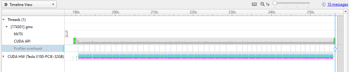
Nsight Systems uses level of detail (LOD) scaling to show you how much GPU usage is under each pixel on the timeline. However, at this zoom level, the data is way too dense to see real patterns. Zooming in reveals the granularity of what Nsight Systems captured.
Likewise, there is information about the GPU activity, but details are organized under drop-downs. Expand the GPU line to reveal information about streams and contexts.
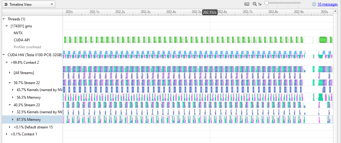
In Figure 2, you can start to see a repetitive pattern of memory transfers and kernel activity on the GPU. Repetitive patterns are normal, but you can also see that a lot of time is being spent on memory transfers. There are gaps in the GPU activity that indicate opportunities for improvement.
Figure 3 zooms in further to 0.1 sec clock time.
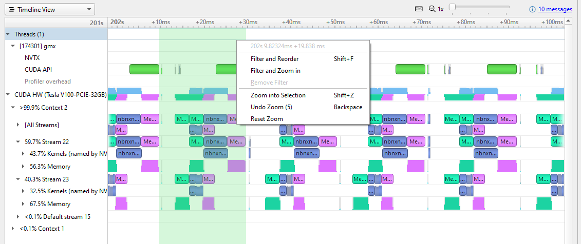
At this resolution, you can clearly see the pattern of activity on the GPU. In each repetition, there is a host-to-device memory transfer (green), some kernel work (blue), and then a memory transfer back to the host (magenta). You can also see the pause after each kernel is run, before the new memory transfer starts.
Figure 3 shows shift-dragging across a single iteration, from the end of the previous device-host transfer to the end of this iteration’s device-host transfer (the selection marked in green). Right-clicking here brings up the menu, and you can zoom in to isolate this iteration.
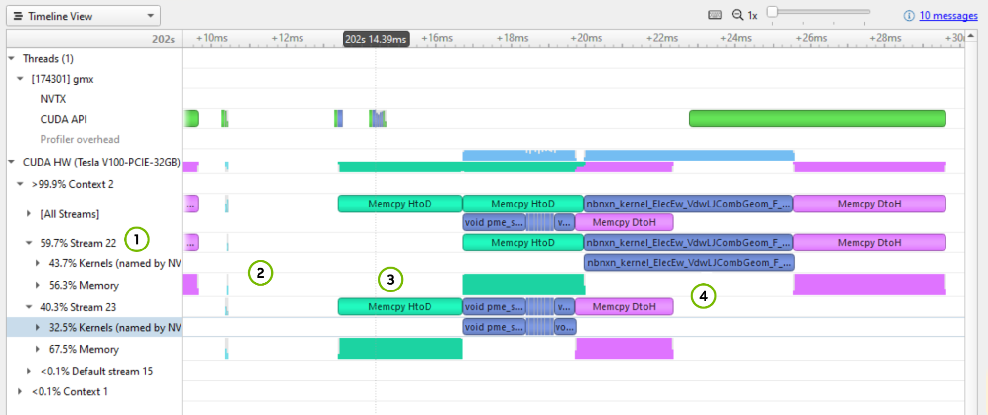
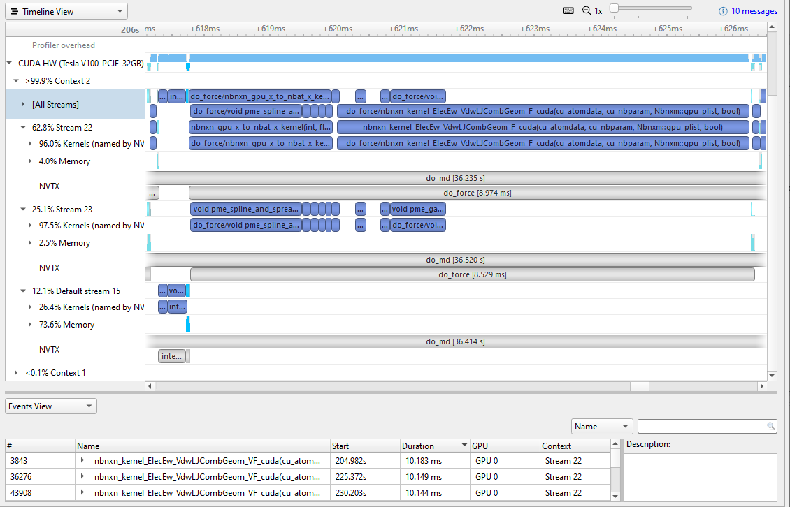
A few things marked on Figure 4 to point out:
- The [All Streams] row is an amalgamation of the streams. Focus on the breakdown, and notice that there is one active context with two active streams (Stream 22 and 23) and that the Default stream is inactive. Each stream is spending more than half of its time on memory transfers. This high percentage is a strong indication that you must optimize the size of memory transfers and consider moving them to the default stream.
- The iteration takes ~19 ms, but 3 ms of that time is in an empty gap between chunks of activity. This implies that there is a ~17% speedup waiting to be captured. A good next step would be to run a CPU profile to check for a programmatic reason for the pause.
- Memory transfers are serialized. Stream 23 gets data from the host, while Stream 22 waits, doing no work until it can get its data. The same thing happens after the work is complete.
- The most dominant work kernel is
nbnxn_kernel_ElecEw_VdwLJCombGeom_VF_cuda. I suggest resolving gaps on the CPU and GPU timelines before diving deeper into individual kernels.
To look for the most expensive kernels, right-click the [All Streams] row and choose Show in Events View (Figure 5).
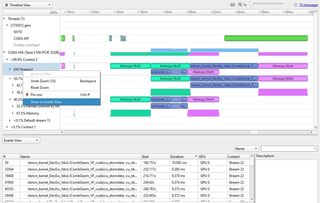
Sorting the Events view by duration reveals the most expensive kernels. Different instances vary a bit, but the most expensive is currently ~10 msec. Clicking on a particular kernel instance highlights all the events that correlate with it on the timeline in cyan.
In Figure 6, a cyan marker on a closed row indicates that something in that row is highlighted. Arrows at the top or left-hand side of the timeline indicate that something highlighted is currently off the screen.
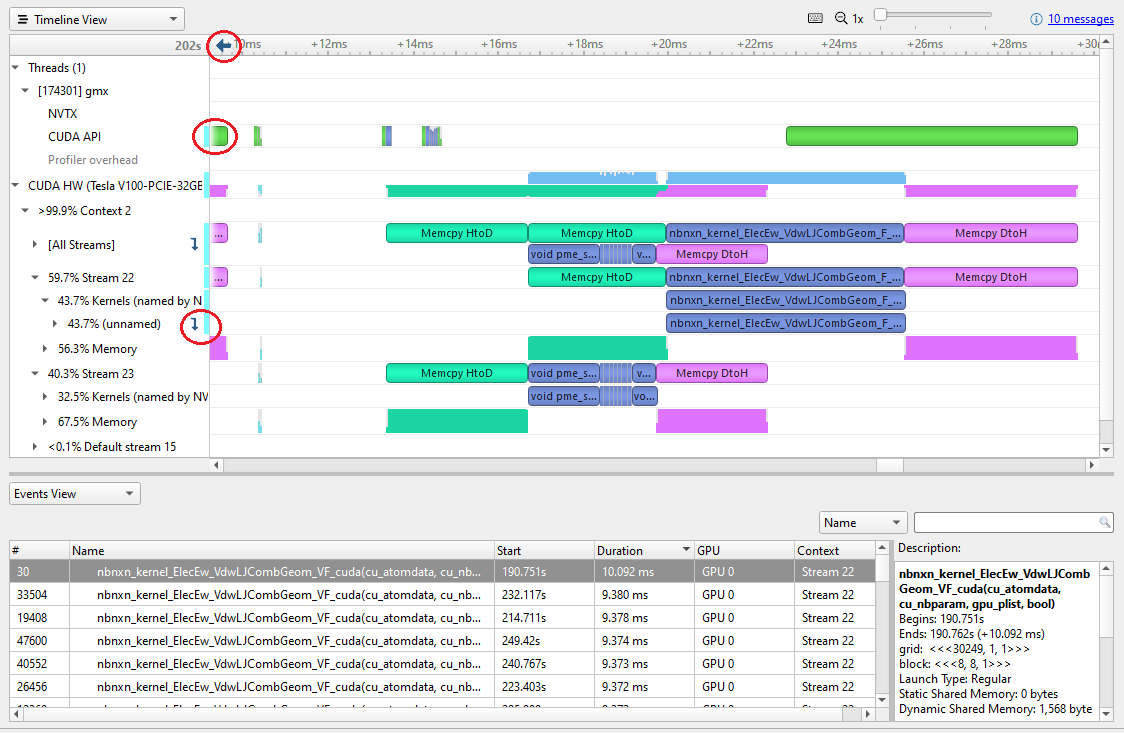
Alternatively, you can right-click in the event table and choose Show Current in Timeline to zoom the timeline to that kernel.
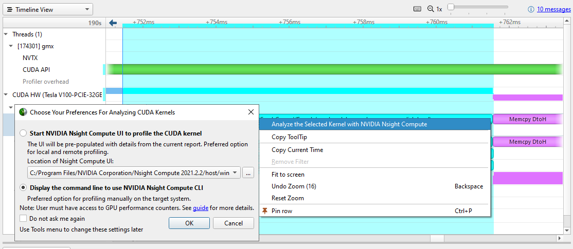
Most of the time, you concentrate on removing timeline gaps and making sure that work is distributed to all CPUs and GPUs before diving into individual kernels. When that time comes, or if kernel performance is out of line with your expectations, you can right-click the kernel of interest and choose Analyze the Selected Kernel with NVIDIA Nsight Compute.
Nsight Compute is a powerful standalone tool for profiling, debugging, and optimizing CUDA kernels. You can launch its user interface or CLI directly from the problematic kernel in Nsight Systems, if it’s installed on your machine.
GROMACS 2020
Improvements were made to GROMACS in collaboration between NVIDIA and the Stockholm GROMACS development team. For more information about the specifics, see Bringing Gromacs Up to Speed on Modern Multi-GPU Systems.
There are a couple of changes that you may notice:
- The
nbnxn_gpu_x_to_nbat_x_kernel is the GPU implementation of a function to convert coordinate data of atoms from “XYZ” into a structure that also has charge in it for data locality: XYZQ. In GROMACS 2019, this was done on the CPU. The 2020 release resized and moved memory transfers to the default stream. - The long kernel
nbnxn_kernel_ElecEw_VdwLJCombGeom_VF_cudanow enables overlapped kernel execution between the two streams.
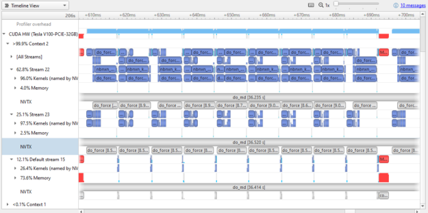
Compare the results in Figure 8 to Figure 3. Both show ~100 msec of wall clock time. As you can see in Figure 8, a lot more of the GPU time is actually doing work. GPU usage has clearly been optimized between versions.
Almost all the memory transfer work has been moved onto the default stream, meaning that the two active streams have little time spent in memory transfer operations (4% and 2.5% compared to over 50% in GROMACS 2019). Small memory transfers have also been combined to larger sizes that still fit in transfer buffers.
Comparing Figure 4 (one work slice of GROMACS 2019) to Figure 9 (one work slice of GROMACS 2020) is not quite a fair comparison. As I mentioned earlier, much of the memory transfer was bundled up and shifted to the default stream. There are several interesting things to note:
- There is much more parallel kernel execution between the two streams.
- The
nbnxn_gpu_x_to_nbat_x_kernel is being run on the GPU before the expensive calculation. Moving this to the GPU instead of the CPU has not only filled up some of the gap time, but it also removed some of the memory transfer overhead. - The expensive kernel,
nbnxn_kernel_ElecEw_VdwLJCombGeom_VF_cuda, has not gotten any faster. The longest instance is still roughly 10 ms. However, because it is more efficiently fed data for this whole iteration of running, that work is reduced to 10 ms instead of the 19 ms in GROMACS 2019.
Now that the gaps are cleared out, nbnxn_kernel_ElecEw_VdwLJCombGeom_VF_cuda is dominating the run time, indicating that your performance tuning journey should move on to that kernel next.
Key takeaways
Improving CUDA kernels is not the first thing that you should do when optimizing GPU code. Improving memory utilization and making sure that the GPU is “fed” enough makes the most immediate impact.
This can be especially important when initially refactoring for GPU or when moving to new generations of GPU hardware. If the GPU is starved for work, you will never realize the performance gains available.
Ready to get started?
This is just the beginning of all the system performance information that Nsight Systems has to offer.
NVIDIA Nsight Systems is available from the NVIDIA CUDA ToolKit public download. You can also obtain the most recent, updated Nsight Systems with enhancements and fixes beyond the version shipping in the NVIDIA CUDA Toolkit on the Nsight Systems page.
For more information about GROMACS, see http://manual.gromacs.org/documentation/.
For other recent posts, see the following:
- Understanding the Visualization of Overhead and Latency in Nsight Systems
- Optimizing DX12 Resource Uploads to the GPU Using CPU-Visible VRAM
For a full list of posts, videos, and other tutorials, see the Other Resources section of the Nsight Systems documentation.
Have a question? Post it to the NVIDIA forums using NVIDIA Nsight Systems. Drop a message at nsight-systems-feedback@nvidia.com. Or just choose Feedback in the application to let us know what you are seeing and what you think.
 GPUs are specially designed to crunch through massive amounts of data at high speed. They have a large amount of compute resources, called streaming…
GPUs are specially designed to crunch through massive amounts of data at high speed. They have a large amount of compute resources, called streaming multiprocessors (SMs), and an array of facilities to keep them fed with data: high bandwidth to memory, sizable data caches, and the capability to switch to other teams of workers (warps) without any overhead if an active team has run out of data.
Yet data starvation may still occur, and much of code optimization focuses on that issue. In some cases, SMs are starved not for data, but for instructions. This post presents an investigation of a GPU workload that experiences a slowdown due to instruction cache misses. It describes how to identify this bottleneck, as well as techniques for removing it to improve performance.
Recognizing the problem
The origin of this investigation is an application from the domain of genomics in which many small, independent problems related to aligning small sections of a DNA sample with a reference genome need to be solved. The background is the well-known Smith-Waterman algorithm (but that by itself is not important for the discussion).
Running the program on a medium-sized dataset on the powerful NVIDIA H100 Hopper GPU, with 114 SMs, showed good promise. The NVIDIA Nsight Compute (NCU) tool, which analyzes a program’s execution on the GPU, confirmed that the SMs were quite busy with useful computations, but there was a snag.
So many of the small problems composing the overall workload—each handled by its own thread—could be run on the GPU simultaneously that not all compute resources were fully used all the time. This is expressed as a small and non-integral number of waves. Work for the GPU is divided into chunks called thread blocks, and one or more can reside on an SM. If some SMs receive fewer thread blocks than others, they will run out of work and must idle while the other SMs continue working.
Filling up all SMs completely with thread blocks constitutes one wave. NCU dutifully reports the number of waves per SM. If that number happens to be 100.5, it means that not all SMs have the same amount of work to do, and that some are forced to idle. But the impact of the uneven distribution is not substantial. Most of the time, the load on the SMs is balanced. That situation changes if the number of waves is just 0.5, for example. For a much larger percentage of the time, SMs experience an uneven work distribution, which is called the “tail” effect.
Addressing the tail effect
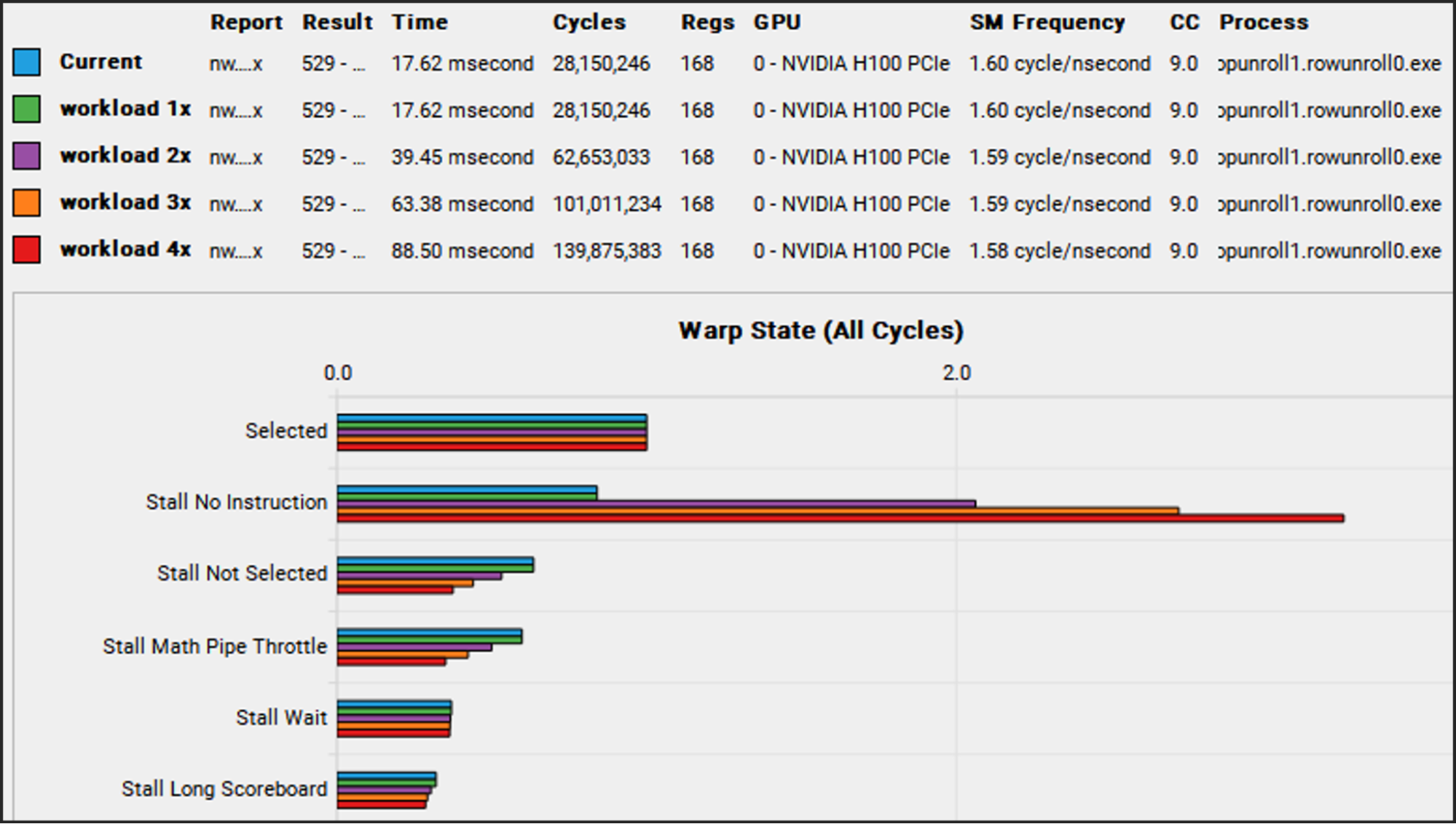
This phenomenon is exactly what materialized with the genomics workload. The number of waves was just 1.6. The obvious solution is to give the GPU more work to do (more threads, leading to more warps of 32 threads each), which is usually not a problem. The original workload was relatively modest, and in a practical environment larger problems need to be completed. However, increasing the workload (1x) by doubling (2x), tripling (3x), and quadrupling (4x) the number of subproblems saw performance deteriorate rather than improve. What could cause this outcome?
The combined NCU report of those four workload sizes sheds light on the situation. In the section called Warp State, which lists the reasons threads cannot make progress, the value for ‘No Instruction’ stands out for increasing significantly with workload size (Figure 1).
‘No Instruction’ means the SMs could not be fed instructions fast enough from memory. ‘Long Scoreboard’ indicates the SMs could not be fed data fast enough from memory. Fetching instructions on time is so critical that the GPU provides a number of stations where instructions can be placed once they have been fetched to keep them close to the SMs. Those stations are called instruction caches, and there are even more levels of them than data caches.
To understand where the instruction caching bottleneck occurred, our team ran the same workloads again, but this time instructed NCU to gather more information than before, using a feature called Metrics. This feature is used to specify a user-defined list of performance counters that are not included in the regular performance reports. In this particular case, a broad array of counters was used related to instruction caches:
gcc__raw_l15_instr_hit, gcc__raw_l15_instr_hit_under_miss, gcc__raw_l15_instr_miss, sm__icc_requests, sm__icc_requests_lookup_hit, sm__icc_requests_lookup_miss, sm__icc_requests_lookup_miss_covered, sm__icc_requests_lookup_miss_to_gcc, sm__raw_icc_covered_miss, sm__raw_icc_covered_miss_tpc, sm__raw_icc_hit, sm__raw_icc_hit_tpc, sm__raw_icc_request_tpc_1b_apm, sm__raw_icc_true_hits_tpc_1b_apm, sm__raw_icc_true_miss, sm__raw_icc_true_miss_tpc, sm__raw_icc_unlock_all_tpc, sm__raw_l0icache_hits_sctlall, sm__raw_l0icache_requests_sctlall, sm__raw_l0icache_requests_to_icc_sctlall, smsp__l0icache_fills, smsp__l0icache_requests, smsp__l0icache_requests_hit, smsp__l0icache_requests_miss, smsp__raw_l0icache_hits, smsp__raw_l0icache_requests_to_icc
The result is that of all the measured quantities, the relatively costly icc cache misses, in particular, increase disproportionately with increasing workload size (Figure 2). The icc cache is an instruction cache that resides in the SM itself and is very close to the actual instruction execution engine.
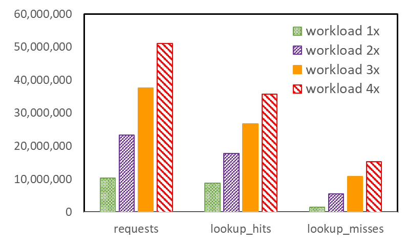
The fact that icc misses increase so quickly implies that, first, not all instructions in the busiest part of the code fit in icc. Second, the need for more different instructions increases as the workload size increases. The reason for the latter is somewhat subtle. Multiple thread blocks, composed of warps, reside on the SM simultaneously, but not all warps execute simultaneously.
The SM is internally divided into four partitions, each of which can generally execute one warp instruction per clock cycle. When a warp is stalled for any reason, another warp that also resides on the SM can take over. Each warp can execute its own instruction stream independently from other warps. At the start of the main kernel in this program, warps running on each SM are mostly in sync. They start with the first instruction and keep chugging along.
However, they are not explicitly synchronizing, and as time goes on and warps take turns idling and executing, they will drift further and further apart in terms of the instructions they execute. This means that a growing set of different instructions must be active as the execution progresses, and this in turn means that the icc overflows more frequently. Instruction cache pressure builds, and more misses occur.
Solving the problem
The gradual drifting apart of the warp instruction streams cannot be controlled, except by synchronizing the streams. But synchronization typically reduces performance, because it requires warps to wait for each other when there is no fundamental need. However, decreasing the overall instruction footprint can be attempted, such that instruction spilling from icc occurs less frequently, and perhaps not at all.
The code in question contains a collection of nested loops, and most of the loops are unrolled. Unrolling improves performance by enabling the compiler to:
- Reorder (independent) instructions for better scheduling
- Eliminate some instructions that can be shared by successive iterations of the loop
- Reduce branching
- Allocate different registers to the same variable referenced in different iterations of the loop, to avoid having to wait for specific registers to become available
Unrolling loops brings many benefits, but it does increase the number of instructions. It also tends to increase the number of registers used, which may depress performance, because fewer warps may reside on the SMs simultaneously. This reduced warp occupancy comes with less latency hiding.
The two outermost loops of the kernel are the focus. Practical unrolling is best left to the compiler, which has myriad heuristics to generate good code. That is, the user expresses that there is an expected benefit of unrolling by using hints, called pragmas in C++, before the top of the loop. These take the following form:
#pragma unroll XWhere X can be blank (canonical unroll), the compiler is only told that unrolling may be beneficial, but is not given any suggestion how many iterations to unroll. Or it can be (n), where n is a positive number that suggests unrolling in groups of n iterations. For convenience, the following notation has been adopted. An unroll factor of 0 means no unroll pragma at all, an unroll factor of 1 means an unroll pragma without any number (canonical), and an unroll factor of n that is larger than 1 means:
#pragma unroll (n)The next experiment comprises a suite of runs in which the unroll factor varies between 0 and 4 for both levels of the two outermost loops in the code, producing a performance figure for each of the four workload sizes. Unrolling by more is not needed because experiments show that the compiler does not generate different code for higher unroll factors for this particular program. Figure 3 shows the outcome of the suite.
The top horizontal axis shows unroll factors for the outermost loop (top level). The bottom horizontal axis shows unroll factors for the second-level loop. Each point on any of the four performance curves (higher is better) corresponds to two unroll factors, one for each of the outermost loops as indicated on the horizontal axes.
Figure 3 also shows, for each instance of unroll factors, the size of the executable in units of 500 KB. While the expectation might be to see increasing executable sizes with each higher level of unrolling, that is not consistently the case. Unroll pragmas are hints that may be ignored by the compiler if they are not deemed beneficial.
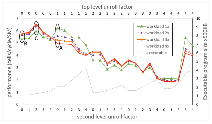
Measurements corresponding to the initial version of the code (indicated by the ellipse labeled A) are for the canonical unrolling of the top-level loop, and no unrolling of the second-level loop. The anomalous behavior of the code is apparent, where larger workload sizes lead to poorer performance, due to increasing icc misses.
In the next isolated experiment (indicated by the ellipse labeled B), attempted before the full suite of runs, neither of the outermost loops is unrolled. Now the anomalous behavior is gone and larger workload sizes lead to the expected better performance. However, absolute performance is reduced, especially for the original workload (1x) size. Two phenomena, revealed by NCU, help explain this result. Due to the smaller instruction footprint, icc misses have dropped virtually to zero for all sizes of the workload. However, the compiler assigned a relatively large number of registers to each thread, such that the number of warps that can reside on the SM is not optimal.
Doing the full sweep of unroll factors suggests that the experiment in the ellipse labeled C is the proverbial sweet spot. It corresponds to no unrolling of the top-level loop, and unrolling by a factor of 2 of the second-level loop. NCU still shows virtually no icc misses, and a reduced number of registers per thread, such that more warps can fit on the SM than in experiment B, leading to more latency hiding.
While absolute performance of the smallest workload still lags by that of experiment A, the difference is not much, and larger workloads fare increasingly better, leading to the best average performance across all workload sizes.
Conclusion
Instruction cache misses can cause performance degradation for kernels that have a large instruction footprint, which is often caused by substantial loop unrolling. When the compiler is put in charge of unrolling through pragmas, the heuristics it applies to the code to determine the best actual level of unrolling are necessarily complicated and are not always predictable by the programmer. It may pay to experiment with different compiler hints regarding loop unrolling to arrive at the optimal code with good warp occupancy and reduced instruction cache misses.
It worked like magic. Computer vision algorithms running in a data center saw that a disease was about to infect a distant wheat field in India. Sixteen days later, workers in the field found the first evidence of the outbreak. It was the kind of wizardry people like Vinay Indraganti call digital transformation. He’s practiced Read article >
A trio of top scientists is helping lead one of the most ambitious efforts in the history of computing — building a digital twin of Earth. Peter Bauer, Bjorn Stevens and Francisco “Paco” Doblas-Reyes agree that a digital twin of Earth needs to support resolutions down to a kilometer so a growing set of users Read article >
When making financial decisions, it’s important to look at the big picture — say, one taken from a drone, satellite or AI-powered sensor. The emerging field of spatial finance harnesses AI insights from remote sensors and aerial imagery to help banks, insurers, investment firms and businesses analyze risks and opportunities, enable new services and products, Read article >
Pre-training visual language (VL) models on web-scale image-caption datasets has recently emerged as a powerful alternative to traditional pre-training on image classification data. Image-caption datasets are considered to be more “open-domain” because they contain broader scene types and vocabulary words, which result in models with strong performance in few- and zero-shot recognition tasks. However, images with fine-grained class descriptions can be rare, and the class distribution can be imbalanced since image-caption datasets do not go through manual curation. By contrast, large-scale classification datasets, such as ImageNet, are often curated and can thus provide fine-grained categories with a balanced label distribution. While it may sound promising, directly combining caption and classification datasets for pre-training is often unsuccessful as it can result in biased representations that do not generalize well to various downstream tasks.
In “Prefix Conditioning Unifies Language and Label Supervision”, presented at CVPR 2023, we demonstrate a pre-training strategy that uses both classification and caption datasets to provide complementary benefits. First, we show that naïvely unifying the datasets results in sub-optimal performance on downstream zero-shot recognition tasks as the model is affected by dataset bias: the coverage of image domains and vocabulary words is different in each dataset. We address this problem during training through prefix conditioning, a novel simple and effective method that uses prefix tokens to disentangle dataset biases from visual concepts. This approach allows the language encoder to learn from both datasets while also tailoring feature extraction to each dataset. Prefix conditioning is a generic method that can be easily integrated into existing VL pre-training objectives, such as Contrastive Language-Image Pre-training (CLIP) or Unified Contrastive Learning (UniCL).
High-level idea
We note that classification datasets tend to be biased in at least two ways: (1) the images mostly contain single objects from restricted domains, and (2) the vocabulary is limited and lacks the linguistic flexibility required for zero-shot learning. For example, the class embedding of “a photo of a dog” optimized for ImageNet usually results in a photo of one dog in the center of the image pulled from the ImageNet dataset, which does not generalize well to other datasets containing images of multiple dogs in different spatial locations or a dog with other subjects.
By contrast, caption datasets contain a wider variety of scene types and vocabularies. As shown below, if a model simply learns from two datasets, the language embedding can entangle the bias from the image classification and caption dataset, which can decrease the generalization in zero-shot classification. If we can disentangle the bias from two datasets, we can use language embeddings that are tailored for the caption dataset to improve generalization.
 |
| Top: Language embedding entangling the bias from image classification and caption dataset. Bottom: Language embeddings disentangles the bias from two datasets. |
Prefix conditioning
Prefix conditioning is partially inspired by prompt tuning, which prepends learnable tokens to the input token sequences to instruct a pre-trained model backbone to learn task-specific knowledge that can be used to solve downstream tasks. The prefix conditioning approach differs from prompt tuning in two ways: (1) it is designed to unify image-caption and classification datasets by disentangling the dataset bias, and (2) it is applied to VL pre-training while the standard prompt tuning is used to fine-tune models. Prefix conditioning is an explicit way to specifically steer the behavior of model backbones based on the type of datasets provided by users. This is especially helpful in production when the number of different types of datasets is known ahead of time.
During training, prefix conditioning learns a text token (prefix token) for each dataset type, which absorbs the bias of the dataset and allows the remaining text tokens to focus on learning visual concepts. Specifically, it prepends prefix tokens for each dataset type to the input tokens that inform the language and visual encoder of the input data type (e.g., classification vs. caption). Prefix tokens are trained to learn the dataset-type-specific bias, which enables us to disentangle that bias in language representations and utilize the embedding learned on the image-caption dataset during test time, even without an input caption.
We utilize prefix conditioning for CLIP using a language and visual encoder. During test time, we employ the prefix used for the image-caption dataset since the dataset is supposed to cover broader scene types and vocabulary words, leading to better performance in zero-shot recognition.
 |
| Illustration of the Prefix Conditioning. |
Experimental results
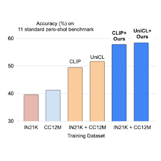
We apply prefix conditioning to two types of contrastive loss, CLIP and UniCL, and evaluate their performance on zero-shot recognition tasks compared to models trained with ImageNet21K (IN21K) and Conceptual 12M (CC12M). CLIP and UniCL models trained with two datasets using prefix conditioning show large improvements in zero-shot classification accuracy.
 |
| Zero-shot classification accuracy of models trained with only IN21K or CC12M compared to CLIP and UniCL models trained with both two datasets using prefix conditioning (“Ours”). |
Study on test-time prefix
The table below describes the performance change by the prefix used during test time. We demonstrate that by using the same prefix used for the classification dataset (“Prompt”), the performance on the classification dataset (IN-1K) improves. When using the same prefix used for the image-caption dataset (“Caption”), the performance on other datasets (Zero-shot AVG) improves. This analysis illustrates that if the prefix is tailored for the image-caption dataset, it achieves better generalization of scene types and vocabulary words.
 |
| Analysis of the prefix used for test-time. |
Study on robustness to image distribution shift
We study the shift in image distribution using ImageNet variants. We see that the “Caption” prefix performs better than “Prompt” in ImageNet-R (IN-R) and ImageNet-Sketch (IN-S), but underperforms in ImageNet-V2 (IN-V2). This indicates that the “Caption” prefix achieves generalization on domains far from the classification dataset. Therefore, the optimal prefix probably differs by how far the test domain is from the classification dataset.
 |
| Analysis on the robustness to image-level distribution shift. IN: ImageNet, IN-V2: ImageNet-V2, IN-R: Art, Cartoon style ImageNet, IN-S: ImageNet Sketch. |
Conclusion and future work
We introduce prefix conditioning, a technique for unifying image caption and classification datasets for better zero-shot classification. We show that this approach leads to better zero-shot classification accuracy and that the prefix can control the bias in the language embedding. One limitation is that the prefix learned on the caption dataset is not necessarily optimal for the zero-shot classification. Identifying the optimal prefix for each test dataset is an interesting direction for future work.
Acknowledgements
This research was conducted by Kuniaki Saito, Kihyuk Sohn, Xiang Zhang, Chun-Liang Li, Chen-Yu Lee, Kate Saenko, and Tomas Pfister. Thanks to Zizhao Zhang and Sergey Ioffe for their valuable feedback.
 This release offers Unreal Engine, NVIDIA RTX, and neural rendering advancements.
This release offers Unreal Engine, NVIDIA RTX, and neural rendering advancements.
Leading users and industry-standard benchmarks agree: NVIDIA H100 Tensor Core GPUs deliver the best AI performance, especially on the large language models (LLMs) powering generative AI. H100 GPUs set new records on all eight tests in the latest MLPerf training benchmarks released today, excelling on a new MLPerf test for generative AI. That excellence is Read article >
![]() At the heart of the rapidly expanding set of AI-powered applications are powerful AI models. Before these models can be deployed, they must be trained through a…
At the heart of the rapidly expanding set of AI-powered applications are powerful AI models. Before these models can be deployed, they must be trained through a…![]()
At the heart of the rapidly expanding set of AI-powered applications are powerful AI models. Before these models can be deployed, they must be trained through a process that requires an immense amount of AI computing power. AI training is also an ongoing process, with models constantly retrained with new data to ensure high-quality results. Faster model training means that AI-powered applications can be deployed more quickly, speeding time to value.
MLPerf benchmarks1 are standardized and proven measures of AI performance across popular AI use cases. MLPerf Training v3.0 is the latest version of the AI training-focused suite of MLPerf tests, covering computer vision, language, and recommender systems, among others. The latest MLPerf Training v3.0 suite has been updated to incorporate a new large language model (LLM) test based on the GPT-3 175B model, representing generative AI. It also features an updated DLRM test with a substantially larger dataset to better represent modern AI-based recommenders.
In MLPerf Training v3.0, the NVIDIA AI platform powered by the NVIDIA H100 Tensor Core GPU set new performance records, achieving both the highest performance on a per-accelerator basis and delivering the fastest time to train on every benchmark at scale.
In addition, the full software stack used for MLPerf Training v3.0 is publicly available. Both NVIDIA submissions, as well as the joint submissions NVIDIA made with CoreWeave, were made in the available category of MLPerf. All NVIDIA submissions achieved similar or improved performance compared to NVIDIA H100 preview submissions in MLPerf Training v2.1.
This post takes a closer look at the performance delivered by the NVIDIA AI platform and the H100 Tensor Core GPU in MLPerf Training v3.0.
NVIDIA AI and H100 Tensor Core GPU deliver record results
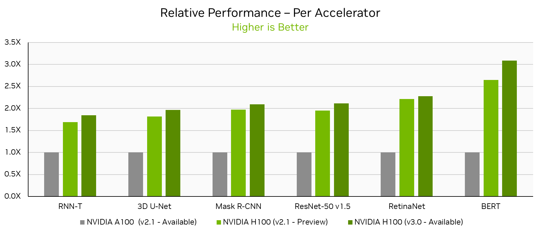
NVIDIA H100 Tensor Core GPUs, which made their MLPerf Training debut just 6 months ago, set new per-accelerator performance records across all MLPerf Training v3.0 workloads. Looking at the NVIDIA single-node DGX H100 results this round, performance increased by up to 17% in just 6 months on the same hardware through software improvements alone. Compared to the NVIDIA A100 Tensor Core GPU submission in MLPerf Training v2.1, the latest H100 submission delivered up to 3.1x more performance per accelerator.
In this round, NVIDIA submitted results using the NVIDIA “Pre-Eos” AI supercomputer on up to 768 H100 GPUs. NVIDIA also made a joint submission with cloud service provider CoreWeave, using up to 3,584 H100 GPUs with the CoreWeave publicly available NVIDIA HGX H100 infrastructure.
Across these submissions, the NVIDIA AI platform with H100 GPUs set new time-to-train records at scale across every workload, including the new LLM workload.
| Benchmark | Max Scale Records(minutes) |
| Large language model (GPT-3) | 10.9 |
| Natural language processing (BERT) | 0.13 (8 seconds) |
| Recommendation (DLRMv2) | 1.61 |
| Object detection, heavyweight (Mask R-CNN) | 1.47 |
| Object detection, lightweight (RetinaNet) | 1.51 |
| Image classification (ResNet-50 v1.5) | 0.18 (11 seconds) |
| Image segmentation (3D U-Net) | 0.82 (49 seconds) |
| Speech recognition (RNN-T) | 1.65 |
MLPerf result IDs: 3.0-2002, 3.0-2075, 3.0-2001, 3.0-2077, 3.0-2066, 3.0-2070, 3.0-2003, 3.0-2065.
The following section details some of the software optimizations behind these results.
NVIDIA software powering MLPerf results
NVIDIA MLPerf Training v3.0 submissions included numerous optimizations that increased performance on existing and updated MLPerf Training workloads, and enabled excellent results on the new LLM test.
Large language model
The newly added LLM workload represents a state-of-the-art large language model with 175 billion parameters. Training this model requires full stack craftsmanship, as it stresses every part of an AI supercomputer, including compute, GPU memory bandwidth, and both internode and intranode interconnect capabilities.
In fact, the workload is so demanding that the smallest-scale NVIDIA submission on this workload used 512 of the latest H100 Tensor Core GPUs on the Pre-Eos system, achieving a time to train of 64.3 minutes. Scaling to 768 GPUs on the same Pre-Eos system reduced time-to-train to 44.8 minutes for near-linear scaling efficiency.
NVIDIA and CoreWeave also made joint submissions on the LLM workload using CoreWeave’s NVIDIA HGX H100 infrastructure at several scales, including 768-GPU, 1,536-GPU, and 3,584-GPU submissions. The 768-GPU submission on CoreWeave’s HGX H100 infrastructure delivered nearly identical performance to the 768-GPU Pre-Eos submission, demonstrating that the NVIDIA AI platform delivers great performance in both on-premises and commercially available cloud instances.
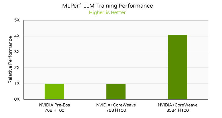
NVIDIA and CoreWeave also submitted LLM results on 3,584 GPUs, delivering a time to train of just 10.9 minutes. This is a more than 4x speedup compared to the 768-GPU submissions on H100, demonstrating 88% performance scaling efficiency even when moving from hundreds to thousands of H100 GPUs.
The software stack used in the MLPerf LLM submission includes NVIDIA NeMo framework combined with the NVIDIA Transformer Engine library, as well as the intelligent use of 8-bit floating-point precision (FP8) on a per-layer basis on NVIDIA H100 GPUs.
BERT
Compared to the prior round, NVIDIA improved per-accelerator H100 performance on the BERT NLP workload by 17%. And NVIDIA and CoreWeave submitted BERT results on up to 3,072 H100 GPUs to deliver a record-setting time to train of 0.134 minutes (a mere 8 seconds).
In order to achieve this performance in publicly available NVIDIA software, the cuDNN library introduced FP8 I/O support in the fused Flash Attention used in the NVIDIA Transformer Engine library. cuDNN fused Flash Attention also supports packed sequence format for Flash Attention I/O, enabling BERT to train at high efficiency without wasting compute on padding tokens. See the cuDNN Developer Guide for more details about cuDNN fused Flash Attention and its documentation.
A summary of the key performance optimizations done in this round for BERT follows:
Data preprocessing
When training models at very large scales, data preprocessing on the CPU may result in significant overhead. To minimize the performance impact of this preprocessing, we overlapped data preprocessing for the next iteration with the computations being performed in the current iteration, reducing iteration time by 3%.
More performant random number generation
In BERT Multi-Head Attention, the online random number generation for the dropout layer starts to become a bottleneck once operations in multi-head attention are fused into a single kernel. This is more pronounced as the Tensor Core throughput of recent NVIDIA GPU architectures has grown faster than the random number generation speed.
To reduce the random number generation bottleneck, we introduced an optimization that uses a comparison of lower precision integer format (8-bit instead of 32-bit) in this MLPerf round, increasing random number generation throughput by 4x. In particular, instead of converting the random 128-bit integer that is produced by the random number generator to four 32-bit integers, we convert it to 16 8-bit integers. This optimization substantially reduces the overhead of random number generation in the multi-head attention block, and results in a 4% end-to-end performance improvement in the application for single-node submission. This optimization does not impact the accuracy or the output quality of the model.
CUDA Graphs
In this submission, we enabled CUDA Graphs for large batch scenarios like training on eight GPUs, through graph-capture support in cuDNN fused Flash Attention and Transformer Engine library, which required carefully handling seed and offset variables of random number generator in multi-head attention.
Furthermore, through optimizations we have reduced conversions between FP16 and FP8 formats and enabled new fused kernels. These optimizations combined boost single-node performance on BERT by 17% compared to the H100 preview submission in MLPerf Training v2.1.
ResNet-50 v1.5
In MLPerf Training v3.0, NVIDIA and CoreWeave made submissions using up to 3,584 H100 Tensor Core GPUs, setting a new at-scale record of 0.183 minutes (just under 11 seconds). Additionally, H100 per-accelerator performance improved by 8.4% compared to the prior submission through software improvements.
In this round, key improvements on the ResNet-50 v1.5 workload include the following:
Faster GroupBatchNorm with NVSHMEM
In this round, we implemented a faster GroupBatchNorm kernel using the NVIDIA NVSHMEM library and reducing inter-GPU communication latency by more than 5x. This new kernel is also able to make use of the high-bandwidth, inter-GPU NVIDIA NVLink interconnect to accelerate communication. This optimization resulted in an end-to-end speedup of 6% in the largest scale submission.
cuDNN kernels
The NVIDIA cuDNN team developed significantly improved convolution kernels that leverage the much faster Tensor Core throughput of the NVIDIA H100 GPU. These kernels led to 5% higher end-to-end performance in both single-node and efficient-scale submissions.
RetinaNet
NVIDIA submitted results on RetinaNet using up to 768 NVIDIA H100 Tensor Core GPUs, achieving a new performance record for the benchmark of just 1.51 minutes. Per-accelerator performance was also enhanced compared to the prior submission.
Optimizations of this round to achieve these results include:
Support for FP32 Master Weights in the Optimizer
The NVIDIA RetinaNet submission in MLPerf Training v3.0 used PyTorch Automatic Mixed Precision (AMP) to leverage the higher throughput that the NVIDIA H100 GPU provides for lower precision data types, like FP16.
However, as model parameters are still maintained in FP32, PyTorch AMP inserts dynamic type casting operations to convert between FP16 and FP32 data types while carrying out tensor operations in the lower precision.
To avoid this overhead, the optimizer maintains a separate set of model parameters stored in FP32 called “master weights.” The model parameters can now be cast entirely to FP16, avoiding the insertion of dynamic type casting operations. The optimizer can update the master weights using the FP16 gradients obtained during the backward pass. This optimization boosted training performance by 10%.
Data preprocessing
The NVIDIA RetinaNet submission uses the NVIDIA Data Loading Library (DALI), a portable, open-source library for decoding and augmenting images, videos, and speech to accelerate deep learning applications.
In MLPerf Training v3.0, the NVIDIA submission used DALI for both data loading and preprocessing of variable-sized images in the dataset. By profiling our large-scale training runs using NVIDIA Nsight Systems, we observed that memory reallocation operations in DALI occur at different times for different processes in the training process, leading to delays in training iterations.
Memory management operations in the DALI image decoder were one primary cause of jitter. These were removed by providing a hint to the largest image size in the dataset—an optimization that boosted performance by 10%.
Optimizations in cuDNN
The cuDNN library has been updated with enhanced kernels that better use the NVIDIA H100 fourth-generation Tensor Cores. These kernels increased the performance of convolutions in our RetinaNet submission, particularly for the smaller-sized ones that are key to at-scale performance, leading to up to 7.5% higher training throughput compared to our prior submission.
3D U-Net
NVIDIA submitted results on 432 NVIDIA H100 Tensor Core GPUs, achieving a new record for the benchmark of 0.82 minutes (49 seconds) to train. Per-accelerator performance on H100 also improved by 8.2% compared to the prior round.
To achieve excellent performance at scale, a faster GroupBatchNorm kernel was one key optimization.
In our largest scale 3D U-Net submission, the instance normalization operation in the neural network needs to perform a reduction of the tensor mean and variance across four GPUs. By using a faster GroupBatchNorm kernel to implement instance normalization, we delivered a 1.5% performance increase.
Mask R-CNN
This round, NVIDIA submitted results on Mask R-CNN using up to 384 H100 GPUs, achieving a new record time to train of 1.47 minutes. Per-accelerator performance also improved by 6.1% compared to the previous submission through software optimizations.
Optimizations this round focused on reducing CPU bottlenecks to ensure that the capabilities of the powerful H100 GPUs were better used.
Faster evaluation
The evaluation process computes the score after inference results have been gathered on a single rank. Since the H100 GPU is able to train significantly faster than the prior-generation A100 GPU, evaluation became a significant performance bottleneck.
In this round, each individual inference result is encoded as JSON (corresponding to a single prediction for each image) before gathering the results on a single rank. After the results were gathered, JSON strings for collections of inference results were formed by concatenating strings from the initial JSON encoding, rather than by decoding and encoding inference results as they passed through the scoring logic. This approach is substantially faster than encoding and decoding and yields a doubling in evaluation speed.
Faster annotations
In previous rounds, annotations—which contain target information for each sample—were loaded from a very large JSON file, a process that took up to 5 seconds. By storing annotations as serialized tensors and loading them, we reduced startup time by more than 80%.
Before annotations can be used for training, they must undergo transformations. Instead of performing these transformations independently for each image, we performed all transformations with a single global kernel as all images undergo the same transformations. This kernel is called once during load and is repeated at the beginning of each epoch.
This optimization reduced the amount of CPU work by nearly 20%. As Mask R-CNN was CPU-limited, training performance increased by almost 20%.
More CUDA graphs
In prior rounds, we CUDA-graphed everything except for loss calculations. We observed that loss calculations accounted for more than 40% of total step time, due to the loss calculation code being CPU bound. By CUDA-graphing the entire model, we improved training throughput by more than 30%.
DLRM_DCNv2
DLRM_DCNv2 is a new benchmark in MLPerf Training v3.0. It replaces the previous DLRM benchmark, with the following updates:
- Multi-hot dataset: The previous DLRM benchmark used a one-hot Criteo dataset. To better represent real-world use and application of recommenders, DLRM_DCNv2 adopts a multi-hot dataset. A multi-hot dataset has been synthesized from the original Criteo one-hot dataset for this purpose.
- Cross layer: The cross layer proposed in the paper DCN V2: Improved Deep and Cross Network and Practical Lessons for Web-scale Learning to Rank Systems is introduced for DLRM_DCNv2.
- Adagrad optimizer: The SGD optimizer used in DLRM is replaced with Adagrad optimizer in DLRM_DCNv2, as Adagrad is more commonly used in real-life recommenders.
Our submission uses the embedding collection in NVIDIA Merlin HugeCTR, which supports many sharding strategies and horizontally fuses embedding operations associated with different embedding shards to deliver excellent performance.
For scale-out training, we employed a hierarchical embedding strategy to leverage the hierarchical nature of the network fabric. This approach resulted in the following benefits:
- Embedding vectors in the same node are reduced by first leveraging NVIDIA NVLink connections to reduce the number of bytes needed to be transferred through the InfiniBand networking connecting GPUs between nodes.
- The reduced embedding vectors are then placed on GPUs that share the same InfiniBand rails as the destination GPU, minimizing transmission latency in rail-optimized systems.
The NVIDIA submission employed a module called input distributor in the embedding collection for performance and flexibility. This module converts the data-parallel input from the data reader to the model-parallel input needed by the embedding operations. To reduce the amount of traffic associated with the input distribution, category filtering is employed to only transmit the categories needed by each GPU. Furthermore, input data is prefetched and distributed to overlap the input distribution of the next iteration with the current iteration, thereby boosting training throughput.
MLPerf Training v3.0 takeaways
The NVIDIA AI platform delivered record-setting performance in MLPerf Training v3.0, highlighting the exceptional capabilities of the NVIDIA H100 GPU and the NVIDIA AI platform for the full breadth of workloads—from training mature networks like ResNet-50 and BERT to training cutting-edge LLMs like GPT-3 175B. The NVIDIA joint submission with CoreWeave using their publicly available NVIDIA HGX H100 infrastructure showcased that the NVIDIA platform and the H100 GPU deliver great performance at very large scale on publicly-available cloud infrastructure.
The NVIDIA platform delivers the highest performance, greatest versatility, and is available everywhere. All software used for NVIDIA MLPerf submissions is available from the MLPerf repository, so you can reproduce these results.
1The MLPerf name and logo are trademarks of MLCommons Association in the United States and other countries. All rights reserved. Unauthorized use strictly prohibited. See www.mlcommons.org for more information.