Author: mcbloom

Orbital edge computing: nanosatellite constellations as a new class of computer system, Denby & Lucia, ASPLOS’20.

Last time out we looked at the real-world deployment of 5G networks and noted the affinity between 5G and edge computing. In true Crocodile Dundee style, Denby and Lucia are entitled to say “that’s not the edge, this is the edge!”. Today’s paper choice has it all: clusters of formation-flying autonomous nanosatellites working in tandem to overcome the physical limitations of space and the limited bandwidth to earth. The authors call this Orbital Edge Computing in contrast to the request-response style of satellite communications introduced with the previous generation of monolithic satellites. Only space system architects don’t call it request-response, they call it a ‘bent-pipe architecture.’

Momentum towards large constellations of nanosatellites requires a reimagining of space systems as distributed, edge-sensing and edge-computing systems.

Satellites are changing!

Satellites used to be large monolithic devices, e.g. the 500kg, $192M Earth Observing-1 (EO-1) satellite. Over the last couple of decades there’s been a big switch to /nanosatellite/ constellations. Nanosatellites are typically 10cm cubes (for the “CubeSat” standard), weigh just a few kilograms, and cost in the thousands of dollars.

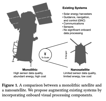
The CubeSat form-factor limits what can be packed into the device and how much power is available. Without higher-risk deployable solar arrays, a cubesat relies on surface-mounted solar panels to harvest energy. This results in peak available power of about 7.1W.

A constellation is a collection of nanosatellites (the space segment) and a collection of on-the-ground transceivers (the ground segment). Constellations today are in the hundreds of nanosatellites, and reconfiguring such a constellation from the ground can take months. Constellations with thousands of nanosatellites are on their way. And it seems we can add satellites to the growing list of things that get finer-grained over time:

Looking forward, we expect deployments of satellites that are even smaller than nanosatellites. Chip-scale or gram-scale satellites (“chipsats”) can be deployed even more numerously and at even lower cost.

The old ground-initiated command-and-control style systems aren’t going to work for these finer-grained systems. To see why, we need to look at some of the physical constraints of computation and communication in space.

Physical constraints

We’ve already seen that nanosatellites have about 7W of power to play with, which they harvest from the environment and store in batteries or supercapacitors. Beyond power, volume is the second key limiting factor, in particular restricting the amount you can pack onboard, and best focal length achievable with cameras.

The Ground Sample Distance (GSD) is the distance on the ground between one pixel and the next in a camera image. It’s a function of orbit altitude, camera focal length, and pixel sensor size. Nanosatellite systems have a GSD of around 3.0m/px. When it comes to GSD, lower is better.

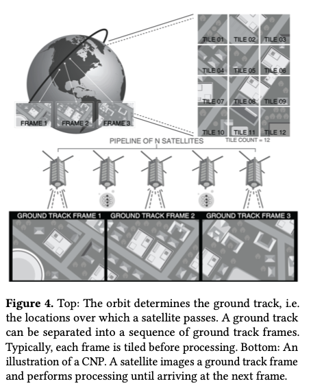
The satellite takes images of a path on the ground called the /ground track/. As it moves around the ground track, the ideal frequency at which to take images is one where each frame is perfectly adjacent to the one before, with no overlapping pixels. This is called the Ground Track Frame Rate (GTFR).

In order to achieve sufficient coverage of a ground track, a satellite or constellation must capture images individually or in aggregate at the GTFR.

In the bent pipe architecture a satellite gathers and stores data until it is near a ground station, and then transmits whatever it has. This results in delays of up to 5.5 hours from capture to receipt of data. A ground station with a 200 Mbit/s downlink datarate can retrieve up to to 15GB of data during a ten minute session. Even under ideal conditions, such a ground station can only support 9 satellites per revolution. It would take 112 ideally positioned stations to support a 1000-node constellation.

Downlink bandwidth increases with receiver gain, which increases with dish diameter on ground stations. Cubesats can’t increase receiver gain in this way due to their limited device size. So uplink data volume is on the order of kilobytes per pass.

That’s not enough bandwidth to download data from thousands of nano-satellites, nor enough to efficiently reconfigure a cluster via the uplink. Satellites are going to have to take responsibility for more decisions on their own, without waiting for commands from a ground station, and they’re going to have to do more onboard processing of data to make better use of the limited downlink bandwidth.

Introducing Orbital Edge Computing (OEC)

Orbital Edge Computing (OEC) is designed to do just that. Coverage of a ground track and processing of image tiles is divided up between members of a constellation in a computational nanosatellite pipeline (CNP).

A CNP leverages existing formation flying techniques to orbit in a fixed configuration, parallelizing data collection and processing across a constellation.

With onboard image processing to identify interesting data, it might be possible to reduce 15GB of raw data down to about 0.75GB that needs to be sent to the ground station. This would take just 30s at 200 Mbit/s. Rather than servicing only 9 satellites per revolution, a ground station could then service 185. The particular form of local processing depends on the application, but it could include for example CNN-based image classification, object detection, segmentation, or even federated machine learning. The general scheme of only sending the interesting parts of the data is known as intelligent early discard.

OEC nanosatellites also run local software for autonomous control, modelling the satellite’s position in time and space, and achievable bitrate, to determine when to communicate and what to communicate (raw data or processed images). This removes the dependence on command-and-control structures initiated at the ground station and sent over the precious uplink bandwidth.

The unique characteristics of OEC systems stem from the astrodynamics that govern them, giving rise to fundamental differences compared to terrestrial edge computing systems.

Formation flying, and formation processing

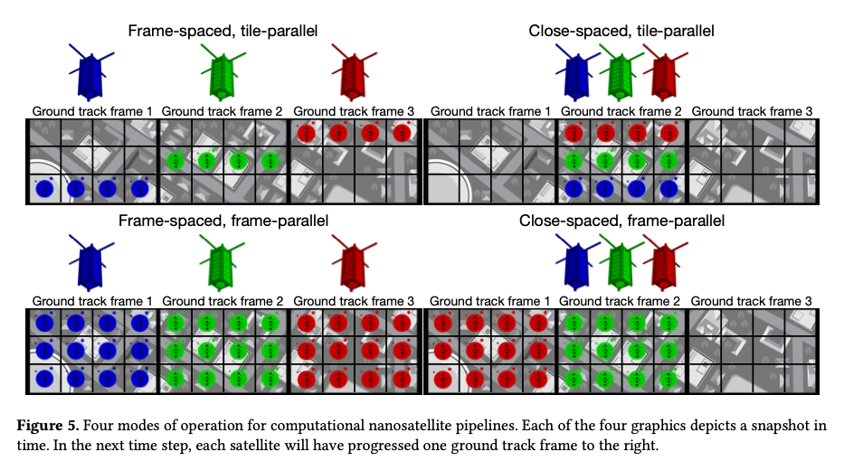
The authors explore two different options for nanosatellite formations with respect to ground track frames (GTFs), and two different options for parallel processing of images. Combined, this results in four different possible OEC configurations.

In a frame-spaced formation the nanosatellites are placed exactly one GTF apart in distance. (My mental model is a sliding window with an array of read heads, so that multiple GTFs can be read in parallel your mileage may vary!). An interesting variant of frame-spacing is orbit spacing which distributes satellites evenly across an orbit giving improved communication opportunities.

A close-spaced formation of nanosatellites packs the nanosatellites as close together as possible, such that the end-to-end pipeline distance between the satellites is less than the length of one GTF.

Whether frame-spaced or close-spaced, there are two options for how each satellite processes an image frame. Consider an image divided up into a set of tiles. With frame-parallel processing each nanosatellite processes all the tiles in each frame. With tile-parallel different tile segments are assigned to different satellites, which then process only their own tiles.

Computing on the edge with cote

These ideas are all packaged together in cote, “the first full-system model for orbital edge computing.” cote has two main components: a pre-mission simulation library, and an online autonomous control library ( cote-lib) to be included in nanosatellite software stacks.

cote-lib runs continuously in the background on an OEC device, explicitly modeling ground station available… [it] enables an OEC satellite to adapt to changing orbit and power conditions in real-time; such fine-grained adaptation is impossible with high-latency bent-pipe terrestrial control.

cote tracks time using Universal Time (UT1), which measure the rotation of the earth relative to distant astronomical objects. It supports three different coordinate frames: Earth-centered inertial (ECI), latitude, longitude and height (LLH), and south, east, z (SEZ). It’s important to model the true oblate nature of the Earth as it matters when establishing communication links via ground satellites with narrow high-gain antenna beams.

Given time and position, cote can use orbital mechanics to model the state of a satellite relative to the rotating earth. The simplified general perturbation model (SGP4) is used as the orbital mechanics engine. SPG4 is the GPS of space!

Understanding where it is relative to the Earth enables cote to model the maximum achievable bitrate for downlink, crosslink, and uplink channels at any given point in time. This can be used to plan when and what to communicate back to earth.

Evaluation

I’m running out of space to cover the evaluation section in any depth, so here are the highlights:

• “Bent pipes are fundamentally unscalable using a constellation of 250 nanosatellites in a $97.3^o$ inclination orbit.”
• Frame-spaced and orbit-spaced constellations downlink the most data, due to the reduction in downlink contention from their spacing.
• Close-spaced constellation have much lower effective bandwidth, but also much lower latency. This is especially marked in the tile-parallel scheme, where the latency reduction for close-spacing is 617x!
• Enabling intelligent early discard can reduce the number of required ground stations by 24x.

We show that an OEC architecture can reduce ground infrastructure over 24x compared to a bent-pipe architecture, and we show that pipelines can reduce system edge processing latency over 617x.

There’s loads of good stuff in this paper that I didn’t have the space to cover here, so if you’re at all interested in this topic I highly recommend checking it out.

Bias in word embeddings, Papakyriakopoulos et al., FAT*’20

There are no (stochastic) parrots in this paper, but it does examine bias in word embeddings, and how that bias carries forward into models that are trained using them. There are definitely some dangers to be aware of here, but also some cause for hope as we also see that bias can be detected, measured, and mitigated.

…we want to provide a complete overview of bias in word embeddings: its detection in the embeddings, its diffusion in algorithms using the embeddings, and its mitigation at the embeddings level and at the level of the algorithm that uses them.

It’s been shown before (‘Man is to computer programmer as woman is to homemaker?’) that word embeddings contain bias. The dominant source of that bias is the input dataset itself, i.e. the text corpus that the embeddings are trained on. Bias in, bias out. David Hume put his finger on the fundamental issue at stake here back in 1737 when he wrote about the unjustified shift in stance from describing what is and is not to all of a sudden talking about what ought or ought not to be. The inputs to a machine learning model are a description of what is. If we train a model on them within thinking, the outputs of the model will treat what is as if it were what ought to be. We have made a sophisticated machine for reinforcing the status quo, warts and all.

When it comes to word embeddings this effect can be especially powerful because the embeddings isolate the words from the contexts in which they were originally used, leaving behind a static residue of bias:

…the projection of words in a mathematical space by the embeddings consolidates stereotyping and prejudice, assigning static properties to social groups and individuals. Relations are no longer context-dependent and dynamic, and embeddings become deterministic projections of the bias of the social world. This bias is diffused into further algorithms unchanged, resulting in socially discriminative decisions.

The authors proceed in the following manner:

• Firstly, they train one set of word embeddings based on the complete German wikipedia, and another set based on Facebook and Twitter content relating to the six main political parties in Germany. The training is done using GloVe. To be able to compare these word embeddings (by placing them both within the same vector space), they then find the linear transformation matrix that places all words from one into the vector space of the other with minimal translation. Since the translation is linear, the normalised distance between words does not change and hence any bias is preserved.
• They then measure bias in the trained embeddings
• Having demonstrated that the word embeddings do indeed contain bias, the next step is to see if a model trained using these word embeddings exhibits bias in its outputs (which they show it does).
• Given the resulting models does show bias, they then explore mechanisms for mitigating that bias at both the word embedding level and at the level of the final trained classifier.
• Finally, they show how biased word embeddings can actually help us to detect the same biases in new text samples (for example, the output of a language model?).

Measuring bias in word embeddings

Say we want to know whether a word embedding for a concept $c$ has a gender bias. We can take the cosine distance between $c$ and ‘Man’ and subtract the cosine distance between $c$ and ‘Woman’. A non-zero result reveals bias in one direction or the other, and the magnitude of the result tells us the amount of the bias. Since the study is done using the German language, which is gendered, concepts with male and female versions are represented by word pairs. This basic technique is used to assess bias in the trained word embeddings for professions, for Germans vs foreigners, and for homosexual vs heterosexual.

The results show that the trained vectors are more likely to associated women with professions such as nursing and secretarial work, whereas men are associated with roles such as policemen and commanders. Germans are linked to positive sentiments such as charm and passion, cooperation and union, while foreigners are generally linked to concepts such as immigration, law, and crime. Homosexuals are related to roles such as hairdresser or artist, and heterosexuals to blue collar professions and science. Homosexuality was associated with negative sentiments, and heterosexuality with positive ones.

Summaries of the most extremely biased words in both the Wikipedia and social media data sets are given in the tables below.

[the] results illustrate that word embeddings contain a high level of bias in them in terms of group stereotypes and prejudice. The intergroup comparison between sexes, populations, and sexual orientations revealed the existence of strong stereotypes and unbalanced evaluation of groups. Although Wikipedia contained a stronger bias in terms of stereotypes, social media contained a higher bias in terms of group prejudice.

Do biased word embeddings lead to biased models?

The authors trained a model that took a word embedding as input and predicted whether that word has a positive or negative sentiment. To assess bias in the trained model, the authors fed names as inputs with the expectation that in the absence of bias, names should have a zero sentiment score as they are polarity independent. The chosen names were stereotypical first names for nine population groups: German, Turkish, Polish, Italian, Greek, French, US American, Russian, and Arabic. The authors also compared male and female names.

The study illustrated the use of biased word embeddings results in the creation of biased machine learning classifiers. Models trained on the embeddings replicate the preexisting bias. Bias diffusion was proved both for sexism and xenophobia, with sentiment classifiers assigning positive sentiments to Germans and negative sentiments to foreigners. In addition, the amount of polarity for men and women in the embeddings was diffused unaltered into the models.

Mitigating bias

The authors investigate two different methods for bias mitigation in the sentiment classifier:

1. Removing bias at the individual word embedding level (by making theoretically neutral words orthogonal to the sentiment vector, where the sentiment vector is e.g. good – bad, positive – negative etc.).
2. Removing bias at the level of the classifier by adjusting the linear hyperplane learned by the linear SVM classifier, such that this plane is orthogonal to the sentiment vector.

While both methods reduce bias in the resulting classifications, the classifier-level correction is much more effective, as can be seen in the following figure.

This is because correcting embeddings for a theoretically neutral set of words still leaves other potential biases in place that weren’t corrected for. The classifier is good at finding these!

…the classifier learns further associations between the vectors, which are not taken into consideration when debiasing at the embeddings level… Hence, we show that debiasing at the classifier level is a much better and safer methodology to follow.

Detecting bias in text

The authors created a dataset containing an equal number of sexist and non-sexist comments from Facebook pages of German political parties. Then they trained models with LSTM and attention-based architectures to classify comments as sexist or non-sexist. Multiple variants were trained, using random embeddings, the Wikipedia embeddings, the social media embeddings, and embeddings trained on the sexist comments.

The more similar the bias in the embeddings with the target data, the higher the ability of the classifier to detect them.

The attention-based network architecture, when given the sexism embeddings, allowed to freely retrain them, and tested on comments only containing words with embeddings, achieved an accuracy of 92%.

A call to action

The study showed that bias in word embeddings can result in algorithmic social discrimination, yielding negative inferences on specific social groups and individuals. Therefore, it is necessary not only to reflect on the related issues, but also to develop frameworks of action for the just use of word embeddings…

When it comes to generative language models, one possibility that strikes me is to use the model to generate a text corpus, train word embeddings on that corpus, and then analyse them for bias. Any detected bias could then be fed back into the language model training process as a form of negative reinforcement.

An overview of end-to-end entity resolution for big data, Christophides et al., ACM Computing Surveys, Dec. 2020, Article No. 127

The ACM Computing Surveys are always a great way to get a quick orientation in a new subject area, and hot off the press is this survey on the entity resolution (aka record linking) problem. It’s an important part of many modern data workflows, and an area I’ve been wrestling with in one of my own projects.

Entity Resolution (ER) aims to identify different descriptions that refer to the same real-world entity appearing either within or across data sources, when unique entity identifiers are not available.

When ER is applied to records from the same data source it can be used for deduplication, when used to join records across data sources we call it record linking. Doing this well at scale is non-trivial; at its core, the problem requires comparing each entity to every other, i.e. it is quadratic in input size.

An individual record/document for an entity is called an entity description. A set of such descriptions is an entity collection. Two descriptions that correspond to the same real world entity are called matches or duplicates. The general flow of an ER pipeline looks like this:

• Blocking takes input entity descriptions and assigns them to one or more blocks based on blocking keys. The point of blocking is to reduce the number of comparisons that have to be made later on – the key idea is that any two entity descriptions that have a chance of referring to the same real-world entity should end up in the same block under at least one of the blocking keys. Therefore we only have to do more detailed comparisons within blocks, but not across blocks. “The key is redundancy, i.e., the act of placing every entity into multiple blocks, thus increasing the likelihood that matching entities co-occur in at least one block.”
• Block processing then strives to further reduce the number of comparisons that will need to be made by eliminating redundant comparisons that occur in multiple blocks, and superfluous comparisons within blocks.
• Matching takes each pair of entity descriptions from a block and applies a similarity function to determine if they refer to the same real-world entity or not. (In an iterative ER process, matching and blocking may be interleaved with the results of each iteration potentially impacting the blocks).
• Clustering groups together all of the identified matches such that all the descriptions within a cluster refer to the same real-world entity. The clustering stage may infer additional indirect matching relations.

The resulting clusters partition the input entity collections into a set of resolved entities.

ER solutions can be classified along three dimensions:

• Schema-awareness – is there a schema to give structure to the data or not?
• The nature of the matching process – is it based on a comparison of attributes in the entity descriptions, or is there more complex matching going on such as comparing related entities to give further confidence in matching?
• The processing mode – traditional batch (with or without budget constraints), or incremental.

Let’s dive into each of the major pipeline stages in turn to get a feel for what’s involved…

Blocking

There’s a whole separate survey dedicated just to the problem of blocking for relational data, so in this survey the authors focus their attention on blocking for schema-less data. There are lots of different approaches to this:

Classic approaches look at relations and attributes. For example Token Blocking makes one block for each unique token in values, regardless of the attribute. Any entity with that token in the value of any attribute is added to the block. Redundancy positive blocking schemes such as token blocking are those in which the probability that two descriptions match increases with the number of blocks that include both of them. For redundancy neutral schemes this is not the case. An example of a redundancy neutral scheme is Canopy Clustering, which uses token-based blocks, but assigns an entity to a block based on a similarity score being greater than a threshold $t_{in}$. Moreover, if the similarity score exceeds $t_{ex} (> t_{in})$ then the description is not added to any further blocks.

Block processing

As with blocking, there are a multiplicity of approaches to block processing. Block cleaning methods may purge excessively large blocks (as these are likely to be the result of common stop-word tokens and hence less useful for matching) and filter the blocks a given description is present in – for example by removing the description from the largest $r%$ of the blocks it appears in. More sophisticated methods may also split and merge blocks. Dynamic approaches schedule block processing on the fly to maximise efficiency.

Comparison cleaning methods work on redundancy positive block collections. A graph is constructed where nodes are entity descriptions, and there is an edge between every pair of nodes co-located in a block, with an edge weight representing the likelihood of a match, e.g. the number of blocks they are co-located in. Once the graph is constructed, edge-pruning can be used to remove lower weighted edges. There are a variety of strategies both for weighting and for pruning edges. For example, Weighted Edge Pruning removes all edges less than or equal to the average edge weight. After pruning, new blocks are created from the retained edges. Learning-based methods train classifiers for pruning.

Matching

A matching function $M$ takes a pair of entity descriptions and measures their similarity using some similarity function $sim$. If the similarity score exceeds a given threshold they are said to match, otherwise they do not match. In a refinement the match function may also return uncertain for middling scores. The similarity function could be atomic, such as Jaccard similarity, or composite (e.g., using a linear combination of several similarity functions on different attributes). Any similarity measure that satisfies non-negativity, identity, symmetry, and triangle inequality can be used.

Collective based matching processes use an iterative process to uncover new matches as a result of matches already made. Merging-based collective techniques create a new entity description based on merging a matched pair, removing the original paired descriptions. Relationship-based collective techniques use relationships in the original entity graph to provide further similarity evidence. For example, Collective ER…

Collective ER employs an entity graph, following the intution that two nodes are more likely to match, if their edges connect to nodes corresponding to the same entity. To capture this iterative intuitive, hierarchical agglomerative clustering is performed, where, at each iteration, the two most similar clusters are merged, until the similarity of the most similar cluster is below a threshold.

A variety of supervised, semi-supervised, and unsupervised matching techniques have also been developed.

The output of the matching process is a similarity graph with nodes corresponding to descriptions and edges connecting descriptions that matched, weighted by the matching probability.

Clustering

Clustering aims to infer more edges from indirect matching relations, while discarding edges that are unlikely to connect duplicates in favor of edges with higher weights. Hence, its end result is a set of entity clusters, each of which comprises all descriptions that correspond to the same, distinct real-world object.

The simplest approach is just to find Connected Components, but generally more advanced clustering techniques are used. For example, Markov Clustering uses random walks to strengthen intra-cluster edges while weakening inter-cluster ones.

Making it incremental

Section 8 in the survey discusses incremental approaches, but my general takeaway is that these seem rather thin on the ground, and mostly oriented towards assembling the information needed to answer an incoming query on the fly. The exception is Incremental Correlation Clustering which updates the clustering results on the fly based on newly created, updated, and deleted descriptions. All of the discussed approaches require schemas.

Open source ER systems

The survey includes an assessment of open source tools for ER, summarised in the table below.

…we share the view of ER as an engineering task by nature, and hence, we cannot just keep developing ER algorithms in a vacuum. In the Big Data era, we opt for open-world ER systems that allow one to plug-and-play different algorithms and can easily integrate with third-party tools for data exploration, data cleaning, or data analytics.

Seeing is believing: a client-centric specification of database isolation, Crooks et al., PODC’17.

Last week we looked at Elle, which detects isolation anomalies by setting things up so that the inner workings of the database, in the form of the direct serialization graph (DSG), can be externally recovered. Today’s paper choice, ‘Seeing is believing’ also deals with the externally observable effects of a database, in this case the return values of read operations, but instead of doing this in order to detect isolation anomalies, Crooks et al. use this perspective to create new definitions of isolation levels.

It’s one of those ideas, that once it’s pointed out to you seems incredibly obvious (a hallmark of a great idea!). Isolation guarantees are a promise that a database makes to its clients. We should therefore define them in terms of effects visible to clients – as part of the specification of the external interface offered by the database. How the database internally fulfils that contract is of no concern to the client, so long as it does. And yet, until Crooks all the definitions, including Adya’s, have been based on implementation concerns!

In theory defining isolation levels in terms of what the database does on the inside should at least be helpful to database developers – although as we’ll see in actual fact it can be over-constraining – but it leaves the much larger number of database users with a harder task to figure out what that means in terms of the effects visible to their applications.

This paper introduces the first state-based formalization of isolation guarantees. Our approach is premised on a single observation: applications view storage systems as black-boxes that transition through a series of states, a subset of which are observed by applications.

With isolation levels defined in terms of observable states, it becomes immediately clear to application developers what states their applications may observe, and it gives the implementors of storage systems maximum freedom in terms of how they meet the required external guarantees. In case you need any further motivation to dig in, in a panel at the Papers-we-love mini-conference earlier this month, this paper was nominated by Joe Hellerstein as a hidden gem deserving of wide visibility.

A motivating example

I’m going to jump ahead in the paper and start with a motivating example. Alice and Bob are joint owners of linked checking and savings accounts at a bank. The bank allows withdrawals from either account, so long as the combined balance remains positive. A withdrawal transaction is given an account and an amount, checks that the combined balance is sufficient to cover the withdrawal, and then debits the specified account by the specified amount.

Is this system safe (will the application invariants be broken) under snapshot isolation? The classic DSG-based definition of snapshot isolation is that it “disallows all cycles consisting of write-write and write-read dependencies and a single anti-dependency.” I’ll wait…

It might be helpful to know that snapshot isolation permits write-skew, and that write skew anomalies are possible when there are integrity constraints between two or more data items.

But it’s even easier with a state-based definition of snapshot isolation (SI). SI requires all operations in a transaction $T$ read from the same complete database state $S$ (the snapshot from which SI gets its name), and that $S$ precedes the transaction execution. But it does not require that the snapshot state be the most recent database state, and other transactions whose effects $T$ will not observe may have taken place in-between the snapshot state and the time that $T$ commits, so long as they don’t write to keys that $T$ also writes to. This matches the intuitive definition of snapshot isolation most people have. So now we can see that two withdrawal transactions could both start from the same snapshot state, in which e.g. the checking and savings account both have a balance of 30. $T_1$ checks that checking + savings has a balance greater than 40, and withdraws 40 from the checking account. $T_2$ checks that checking + savings has a balance greater than 40, and withdraws 40 from the savings account. But once both transactions have committed, the balance is negative and the application invariant has been violated!

Defining isolation levels in terms of state

A storage system supports read and write operations over a set of keys $K$. The state $s$ of the storage system is a total function from keys to values $V$ (some keys may be mapped to $bot$). A transaction $T$ is a sequence of read and write operations. To keep things simple we assume that all written values are unique. Applying a transaction $T$ to the state $s$ results in a new state $s’$. We say that $s$ is the parent state of $T$. An execution $e$ is a sequence of atomic state transitions.

If a read operation in a transaction returns some value $v$ for key $k$, then the possible read states of that operation are the states in $e$ that happened before the transaction started and where $k=v$. Once a write operation in a transactions writes $v$ to $k$, then all subsequent read operations for $k$ in the same transaction should return value $v$ (and for simplicity, we say that each key can be written at most once in any transaction). The pre-read predicate holds if every read operation has at least one possible read state.

This is all we need to start specifying the semantics of isolation levels.

In a state-based model, isolation guarantees constrain each transaction $T in Large{tau}$ in two ways. First, they limit which states among those in the candidate read sets of the operations in $T$ are admissible. Second, they restrict which states can serve as parent states for $T$.

Read uncommitted

Anything goes – no constraints.

Read Committed

A transaction can commit if the pre-read predicate holds (you only read valid committed values)

Snapshot Isolation

If a given state is a valid read state for all the reads in a transaction, then this state is said to be complete with respect to that transaction.

There are two conditions for a transaction $T$ to commit under SI:

1. There must exist a complete state $s$ wrt. $T$ in the execution history (this will be the snapshot state)
2. For the subset of keys that $T$ writes to, states in the execution history following $s$, up to and including the parent state of $T$, must not contain modifications to those keys. This is known as the no-conflicts condition.

Serializability

A transaction $T$ can commit if its parent state is complete wrt. $T$.

Strict Serializability

Adds to serializability the constraint that the start time of a transaction $T$ must be later than the commit time of the transaction responsible for its parent state. (Things happen in real-time order).

Other

In section 4 you’ll also find state-based definitions of parallel snapshot isolation, and read atomic which I don’t have space to cover here.

The commit tests for each isolation level are summarised in the table below:

Understanding the snapshot isolation family

In section 5.2 Crooks et al. use the state-based lens to examine the family of snapshot based guarantees that have grown up over time, including ANSI SI, Adya SI, Weak SI, Strong SI, Generalized SI, Parallel SI, Strong Session SI, Lazy Consistency (PL-2+) SI, and Prefix-Consistent SI. They find that these definitions can be compared on three dimensions:

1. time: are timestamps logical or based on real-time?
2. snapshot recency: is the snapshot required to contain all transactions that committed before the transaction start time?
3. state-completeness: does the snapshot have to be a complete state, or is a causally consistent state sufficient?

Grouping isolation levels in this way highlights a clean hierarchy between these definitions, and suggests that many of the newly proposed isolation levels are in fact equivalent to prior guarantees.

Revealing performance enhancement opportunities

By removing artificial implementation constraints, definitions in terms of client-observable states gives implementers maximum freedom to find efficient strategies. The classic definition of parallel snapshot isolation (PSI) requires each datacenter to enforce snapshot isolation. This is turn makes PSI vulnerable to slowdown cascades in which a slow or failed node can impact operations that don’t access that node itself (because a total commit order is required across all transactions). The state-based definition shows us that a total order is not required, we only care about the ordering of transactions that the application itself can perceive as ordered with respect to each other. In simulation, the authors found a two orders of magnitude reduction in transaction inter-dependencies using this client-centric perspective.

The last word

[The state-based approach] (i) maps more naturally to what applications can observe and illuminates the anomalies allowed by distinct isolation/consistency levels; (ii) makes it easy to compare isolation guarantees, leading us to prove that distinct, decade-old guarantees are in fact equivalent; and (iii) facilitates reasoning end-to-end about isolation guarantees, enabling new opportunities for performance optimization.

Elle: inferring isolation anomalies from experimental observations, Kingsbury & Alvaro, VLDB’20

Is there anything more terrifying, and at the same time more useful, to a database vendor than Kyle Kingsbury’s Jepsen? As the abstract to today’s paper choice wryly puts it, “experience shows that many databases do not provide the isolation guarantees they claim.” Jepsen captures execution histories, and then examines them for evidence of isolation anomalies. General linearizability and serializability checking are NP-complete problems due to extreme state-space explosion with increasing concurrency, and Jepsen’s main checker, Knossos, taps out on the order of hundreds of transactions.

Databases are in for an ‘Ell(e) of a hard time with the new checker in the Jepsen family though, Elle. From the README:

Like a clever lawyer, Elle looks for a sequence of events in a story which couldn’t possibly have happened in that order, and uses that inference to prove the story can’t be consistent.

The paper describes how Elle works behind the scenes, and gives us a taste of Elle in action. Elle is able to check histories of hundreds of thousands of transactions in just tens of seconds. Which means whole new levels of stress for systems under test.

In the evaluation section we see Elle being used to test two SQL databases (TiDB, YugaByteDB), a document database (Fauna), and a graph database (Dgraph). By now I hardly consider it a plot-spoiler to tell you that it finds (unexpected) anomalies in all of them. You’ll find the details in §6 of the paper, and more information on the collaboration between Jepsen and the respective vendors to find and fix these issues on the Jepsen website.

What do we want from a transaction isolation checker?

An ideal transaction isolation checker would be able to…

• Work with general patterns of transactions (not just specially chosen ones)
• Detect many different types of anomalies, such that multiple isolation levels can be tested
• Provide minimal reproducible bug reports when it does find a violation
• Be efficient, so that large numbers of transactions at high levels of concurrency can be checked
• Only report genuine anomalies (soundness)
• Find all anomalies that exist in a history (completeness)

Elle ticks all the boxes, with the exception of completeness. In practice though, Elle typically does observe enough of a history to detect both cyclic and non-cyclic anomalies when they occur, with a guarantee holding under certain conditions.

Anomalies and the Direct Serialization Graph

Adya et al. gave portable definitions of isolation levels and anomalies in their 2000 paper “Generalized Isolation Level Definitions.” Central to the analysis is the notion of a Direct Serialization Graph (DSG). In a DSG nodes represent transactions, and edges between nodes are dependencies between transactions. There are three different types of edges possible between two transactions $T_i$ and $T_j$.

• a write dependency occurs when $T_j$ overwrites a value previously written by $T_i$.
• a read dependency occurs when $T_j$ reads a value previously written by $T_i$ (ignoring the complications of predicate reads for now)
• an anti-dependency occurs when $T_j$ overwrites a value previously read by $T_i$.

The thing all these have in common is that they imply $T_j$ must follow $T_i$ in any serializable history. From this it follows that any cycle in the DSG means that there cannot be a valid serial history.

If only…

What Knossos does is identify write-read dependencies between transactions, translate these into an integer constraint problem, and feed it to a constraint solver to try and find a legitimate serial history. This works to a point but runs into the state-space explosion issues we touched on earlier with histories on the order of (small numbers of) hundreds of transactions. Moreover, when the constraint solver says “no”, we don’t have any insight into why the constraints couldn’t be solved.

This is all a lot more complex than the cycle checking needed in Adya’s model. For example, in a strongly connected component of a graph, every node in the component is reachable from every other node in the same component. If A is reachable from B, and B is reachable from A, we have a cycle! Tarjan’s strongly connected components algorithm can find the strongly connected components in a graph in linear time!

If only we actually had one of Adya’s Direct Serialization Graphs for a given run, then we’d have the triple benefit of anomaly detection exactly matching the definitions of the anomalies, explainability of the anomalies found in terms of those definitions (show the cycle), and linear runtime.

… there is one significant obstacle to working with an Adya history: we don’t have it. In fact, one may not even exist – the database system may not have any concept of a version order, or it might not expose that ordering information to clients.

Recoverability and traceability

So maybe we don’t have an Adya history out of the box. But can we recover one? That is, are there observations we could make of the running system, that are in our control, that would let us infer an Adya history? We know the nodes in the graph – that’s the set of transactions we submit – and we know the operations within those transactions (the reads and writes), as well as having visibility of commit and abort operations. What we need then, is some way of determining the edges.

If every written value is unique, and we have a scheme that enables mapping unique values back to transactions, then when we read a value (in $T_j$), we can always tell which transaction $T_i$ must have written it. This enables us to find the read dependency edges, a property the authors call recoverability.

For a write dependency though, we need to know the transaction $T_i$ that previously wrote the value $T_j$ is overwriting. Unfortunately that history is lost at the moment the old value is overwritten. Unless… we use a datatype that supports append operations (like a string, with concat, or an array), and we follow the convention that all writes must be appends of recoverable values. Now when we read the value, the full history is contained within it. E.g., we might read the list $[(T_i, 1), (T_j, 2)]$ and know that $T_i$ first wrote the value 1, and $T_j$ subsequently wrote the value 2. This is a property the authors call traceability.

If we’ve got recoverability and traceability then with a bit more work we can also find the anti-dependency edges – we have visibility into the return values of read operations, and we just have to look for traceable writes that append to that read value.

Because the model also includes commit and abort operations, this process additionally enables us to detect dirty updates where a transaction commits a version based on reading uncommitted state, as well as corruptions (garbage reads) where a transaction reads a value that no-one has written!

Inferring Direct Serialization Graphs

An inferred direct serialization graph is a DSG constructed from the inferred dependencies between transactions using the techniques just outlined. There’s one more piece of information we can use too, since we control the processes: if process $P$ performs $T_i$ and then $T_j$ then we know that $T_i$ must come before $T_j$ in the history. Adding in these per-process dependencies means that we can strengthen consistency checking in some cases (e.g. from snapshot isolation to strong session snapshot isolation).

Giving the database the benefit of the doubt

Things get a bit more complicated once we allow for the possibility of in-doubt transactions:

… when a client attempts to commit a transaction, but the result is unknown, e.g. due to a timeout or database crash, we leave the transaction with neither a commit nor abort operation.

Observations made in the presence of in-doubt transactions are said to be indeterminate. The problem then arises that there may be many possible histories compatible with the observation.

Elle provides soundness in the face of this complication by constructing a dependency graph which is a (maximal?) subgraph of every possible history compatible with that observation. If a cycle is detected in the subgraph, than it must exist in all compatible histories.

Putting it altogether

Putting this altogether, Elle can detect cycle-based dependencies (Adya’s G0, G1c, G-single, and G2 cycles), aborted reads, intermediate reads, and dirty updates.

In addition, there are phenomena which Adya et al.’s formalism does not admit, but which we believe (having observed them in real databases) warrant special verification.

These are the aforementioned garbage reads, as well as duplicate writes (the same argument written multiple times) and internal inconsistencies (where a transactions reads a value incompatible with its own prior reads and writes).

I’ve only been able to give a high level appreciation in this post, rest assured the paper itself is precise in its terminology and analysis, as befits the subject matter. If these ideas have caught your interest, it’s well worth reading in full.

The last word

Elle is effective. It has found anomalies in every database we’ve checked, ranging from internal inconsistency and aborted reads to anti-dependency cycles… Unlike solver-based checkers, Elle’s cycle-detection approach produces short witnesses of specific transactions and human-readable explanations of why each witness must be an instance of the claimed anomaly… We believe Elle will make the database industry safer.

Achieving 100 Gbps intrusion prevention on a single server, Zhao et al., OSDI’20

Papers-we-love is hosting a mini-event this Wednesday (18th) where I’ll be leading a panel discussion including one of the authors of today’s paper choice: Justine Sherry. Please do join us if you can.

We always want more! This stems from a combination of Jevon’s paradox and the interconnectedness of systems – doing more in one area often leads to a need for more elsewhere too. At the end of the day, there are three basic ways we can increase capacity:

1. Increasing the number of units in a system (subject to Amdahl’s law).
2. Improving the efficiency with which we can coordinate work across a collection of units (see the Universal Scalability Law)
3. Increasing the amount of work we can do on a single unit

Options 1 and 2 are of course the ‘scale out’ options, whereas option 3 is ‘scale up’. With more nodes and more coordination comes more complexity, both in design and operation. So while scale out has seen the majority of attention in the cloud era, it’s good to remind ourselves periodically just what we really can do on a single box or even a single thread.

Today’s paper choice is a wonderful example of pushing the state of the art on a single server. We’ve been surrounding CPUs with accelerators for a long time, but at the heart of Pigasus‘ design is a really interesting inversion of control – the CPU isn’t coordinating and calling out to the accelerator, instead the FGPA is in charge, and the CPU is playing the support role.

IDS/IPS requirements

Pigasus is an Intrusion Detection / Prevention System (IDS/IPS). An IDS/IPS monitors network flows and matches incoming packets (or more strictly, Protocol Data Units, PDUs) against a set of rules. There can be tens of thousands of these rules, which are called signatures. A signature in turn is comprised of one or more patterns matching against either the header or the packet content, including both exact string matches and regular expressions. Patterns may span multiple packets. So before matching, the IDS/IPS has to reconstruct a TCP bytestream in the face of packet fragmentation, loss, and out-of-order delivery – a process known as reassembly.

When used in prevention mode (IPS), this all has to happen inline over incoming traffic to block any traffic with suspicious signatures. This makes the whole system latency sensitive.

So we need low latency, but we also need very high throughput:

A recurring theme in IDS/IPS literature is the gap between the workloads they need to handle and the capabilities of existing hardware/software implementations. Today, we are faced with the need to build IDS/IPSes that support line rates on the order of 100Gbps with hundreds of thousands of concurrent flows and capable of matching packets against tens of thousands of rules.

Moreover, Pigasus wants to do all this on a single server!

Back of the envelope

One of the joys of this paper is that you don’t just get to see the final design, you also get insight into the forces and trade-offs that led to it. Can you really do all this on a single server??

The traditional approach to integrating FPGAs in IDS/IPS processing is to have the CPU in charge, and offload specific tasks, such as regular expression parsing, to the FPGA. The baseline for comparison is Snort 3.0, “the most powerful IPS in the world” according to the Snort website. In particular, Pigasus is designed to be compatible with Snort rulesets and evaluated using the Snort Registered Ruleset (about 10K signatures). The biggest fraction of CPU time in Snort is spent in the Multi-String Pattern Matcher (MSPM) module, which is used for header and partial string matching.

Using Amdahl’s Law, we can see that even if MSPM were offloaded to an imaginary, infinitely fast accelerator, throughput would increase by only 85% to 600Mbps/core, still requiring 166 cores to reach 100Gpbs.

In fact, whatever module of Snort you try to offload to a hypothetical infinitely fast accelerator, you can never get close to the performance targets of Pigasus. That fixes Pigasus’ first design decision: the FPGA needs to be in charge as the primary compute platform, and the CPU will be secondary in service of it. (FPGAs are chosen because they are both energy efficient and available on SmartNICs).

Having settled on an FPGA-first design, this means that stateful packet processing for matching and reassembly needs to be performed on the FPGA. And that in turn means that the primary design constraint is the amount of FPGA memory available, especially Block RAM (BRAM). The target FPGA for Pigasus has 16MB of BRAM.

Of concern here is the regular expression matching performed by the Full Matcher. Regular expression matching is well studied, but state of the art hardware algorithms don’t reach the performance and memory targets needed for Pigasus. Performing RE matching on the FPGA would consume a lot of memory, and offer only marginal overall performance gains since most packets don’t touch the full matcher. This brings us to another major design decision: regular expression matching will be offloaded from the FPGA to the CPU.

Introducing Pigasus

Putting together everything we’ve learned so far, the overall architecture of Pigasus looks like this:

• The reassembler is responsible for ordering TCP packets. It needs to do this at line rate while maintaining state for 100K flows.
• The multi-string pattern matcher (MSPM) does header matching for all 10,000 rules, and exact string-match filtering to determine which further rules might possibly match.
• If the MSPM indicates a possible match, the packet and rule IDs are sent to the DMA Engine, which farms work out to the CPU for full matching.
• The Full Matcher runs on the CPU, polling a ring buffer populated by the DMA Engine.

To save the precious BRAM for the most performance sensitive tasks (reassembly and MSPM), the packet buffer and DMA Engine use the less powerful eSRAM and DRAM available on the FPGA.

Both the reassembler and MSPM modules required careful design to meet their performance and memory targets.

The reassembler: processing fast and slow

The key objective of our Reassemble is to perform this re-ordering for 100K’s of flows, while operating at 100Gbps, within the memory limitations of the FPGA.

The FPGA hardware really wants to operate in a highly parallel mode using fixed size data structures. This works well until we consider out of order packet arrival. To accomodate out-of-order packets though, a memory dense structure such as a linked list works better.

The solution is to divide the reassembly pipeline into a fast path handling in-order flows using fixed size buffers and constant time operations, and a slow path handling the remaining out of order flows. The constant time operations on the fast path guarantee a processing rate of 25 million packets-per-second, enough to reach the 100Gbps target at 500B+ packets. The slow path can’t take advantage of constant time operations, but fortunately is less often used as most packets arrive in order. It’s also used when inserting new flows.

The fast path, new flow insertion, and out-of-order processing all synchronise over shared flow state using a cuckoo-hashing based hash table design from FlowBlaze.

MPSM: First things first

There are challenges in the design of the MSPM too.

To the best of our knowledge, there are no other hardware or software projects reporting multi-string matching of tens of thousands of strings at 100Gpbs.

Snort 3.0 uses Intel’s Hyperscan library for MSPM. The Hyperscan string matching library is parallelisable and provides an 8x speedup over software state-machine based string matchers. But a simple translation to FPGA would blow the memory budget, requiring about 25MB of BRAM.

By carefully staging the work, Pigasus manages to fit everything into just 2MB of BRAM. This means it even has capacity to do more work in the MSPM stage than Snort itself does, reducing the amount of packets that need to be passed to the full matcher.

At the end of the day, a packet must match all the patterns in a signature for the rule to be triggered. The key insight in Pigasus is that some tests can be done very cheaply in terms of time and memory, while others are more memory intensive. Put this together with the realisation that most packets and most indices don’t match any rules at all and a plan emerges: make a filtering pipeline that progressively narrows. At the start of the pipeline we can afford to run lots of memory-cheap filters in parallel. Only a subset of incoming packets make it past these filters, so we need less of the more memory intensive filters running in parallel behind them to achieve the desired line rate.

Applying this filter first allows us to use fewer replicas of subsequent data structures (which are larger and more expensive), since most bytestream indices have already been filtered out by the string matcher. This enables high (effective) parallelism with a lower memory overhead.

This strategy is so effective that whereas Snort passes a packet to the full matcher if any filter matches, Pigasus is able to test for all string matches and further reduce the fraction of packets that head to the CPU for full-matching to just 5%. This testing is performed in parallel using a bloom-filter like representation, see §5.2 in the paper for details.

Headline results

Our experiments with a variety of traces show that Pigasus can support 100Gbps using an average of 5 cores and 1 FPGA, using 38x less power than a CPU-only approach.

There’s a full evaluation in §6 of the paper which I don’t have space to cover here. The headline is that Pigasus meets its design objectives using 23-200 fewer cores than Snort, and 18-62x less power!

The design of Pigasus is a singular proof point that a seemingly unattainable goal (…) on a single server is well within our grasp… Given the future hardware roadmaps of FPGAs and SmartNICs, we believe that our insights and successes can more broadly inform in-network acceleration beyond IDS/IPS as well.

Helios: hyperscale indexing for the cloud & edge, Potharaju et al., PVLDB’20

Last time out we looked at the motivations for a new reference blueprint for large-scale data processing, as embodied by Helios. Today we’re going to dive into the details of Helios itself. As a reminder:

Helios is a distributed, highly-scalable system used at Microsoft for flexible ingestion, indexing, and aggregation of large streams of real-time data that is designed to plug into relationals engines. The system collects close to a quadrillion events indexing approximately 16 trillion search keys per day from hundreds of thousands of machines across tens of data centres around the world.

As an ingestion and indexing system, Helios separates ingestion and indexing and introduces a novel bottoms-up index construction algorithm. It exposes tables and secondary indices for use by relational query engines through standard access path selection mechanisms during query optimisation. As a reference blueprint, Helios’ main feature is the ability to move computation to the edge.

Requirements

Helios is designed to ingest, index, and aggregate large streams of real-time data (tens of petabytes a day). For example, the log data generated by Azure Cosmos. It supports key use cases such as finding records relating to specific attributes (e.g. for incident support), impact and drill-down analysis, and performance monitoring and reporting. One interesting use case is in support of GDPR right to be forgotten requests, where it becomes necessary to search 10s of billions of streams to find those containing a user’s information.

Incoming streams can have data rates as high as 4TB/minute, with many columns to be indexed (7+ is common) and high cardinality.

System design

A stream table is defined by a loose schema which defines the sources to be monitored (as a SourceList) and indices to be created. For example:

Based on the CREATE STREAM statement, Helios generates an agent executable to be deployed on every machine producing a log that is part of the stream. It also generates an executable to be run on the server-side ingestion machines. The agent process accumulates and chunks incoming data into data blocks (with frequency determined by the CHUNK EVERY clause). Optionally, and central to how Helios handles high volume and velocity ingest at manageable scale and cost, the agent can also perform local processing (parsing, indexing, and aggregation) and send the resulting index entries to the ingestion clusters in a compact format.

Ingestion servers are stateless, running the user-defined dataflow (based on the CREATE SCHEMA statement) to process incoming blocks. Data blocks are stored in a distributed file system, and once acknowledged by the file system, an entry is written into Helio’s progress log. The progress log is used to track the progress of both data ingestion and index building. Secondary index generation (hydration) then happens asynchronously. The resulting index blocks are merged into a global index which maps (column, value) pairs to data block URIs.

The progress log is the only strongly synchronized component in Helios, and is deployed in quorum based rings of 5 servers. There are multiple replicated logs each governing a partition of the data set. In this manner Helios achieves a consistent rate of 55,000 writes/second for metadata persistence.

Indexing

A key factor in Helios’s success is asynchronous index mangement: Helios maintains eventually consistent indexes against the data, but exposes a strongly consistent queryable view of the underlaying data with best-effort index support.

Helios’ index is a multi-level (tree-based) structure that is built in a bottom-up manner. I.e., information is inserted at the leaves, and the index then ‘grows upwards’ through merge and add operations. The authors point out an interesting similarity to learned index structures here: “At the highest level, a learned index tries to learn a function that maps an index search key to the leaf nodes containing the search key. The Helios structure in its generic form performs exactly the same function, with the different that the mapping is not learned from data but composed from the (typically, hash) partitioning functions used by the different index levels.“

Indexing begins by scanning the progress log from the latest checkpoint, with an initial leaf node at the bottom of the tree (level 0) constructed for each chunk. No global order is imposed here, indexed keys are simply packed into leaf nodes based on arrival order. Multiple nodes at the same level may be combined into one using the merge operator in accordance with a merge policy. Just as level 0 watches blocks arrive in the progress log and follows along creating leaf nodes, so the next level up, level 1 watches the progress of leaf nodes arriving at level 0, and creates a higher level index over the leaf nodes by applying the add operator. Level 2 follows the progress of level 1 in a similar manner, and so on for the desired number of levels. The result is an indexing frontier that moves forward across the levels through a per-level watermark.

An index node is a collection of (key, pointers) pairs. The merge operation combines two index nodes $N_1$ and $N_2$ by taking the union of their keys, and for each key the union of the pointers. E.g. if $N_1 = {K_1 mapsto {P_1, P_2}, K_2 mapsto {P_3}}$ and $N_2 = {K_2 mapsto {P_4}}$ then $N_1 oplus N_2 = { K_1 mapsto {P_1, P_2}, K_2 mapsto {P_3, P_4 }}$. Helios uses a size-based merge policy in which two nodes are merged if they are both below a given size threshold.

The add operation creates a new node at one level up containing the union of the keys in the blocks being added, and pointers to the nodes in the level below containing entries for those keys. E.g. $N_1 + N_2 = {K_1 mapsto {P_{N_1}}, K_2 mapsto {P_{N_1}, P_{N_2}}}$. Helios also uses a size-based add policy, in which nodes are added (at higher and higher levels) until the size of the resulting node reaches a configurable threshold.

Note that the resulting structure may contain orphan nodes (shown in grey in the figure above) that do not have any parent in the layer above. This has implications for query processing that we’ll look at shortly.

Index compaction, which also takes place bottom-up, is triggered when a configurable number of data blocks have been processed.

Federated indexing

Our initial approach towards data and index management focused towards bringing in data from all the sources into an ingestion cluster and performing the required post-processing operations (e.g. parsing, indexing, etc.). However, this approach incurs significant costs… The hierarchical/recursive indexing model gives the freedom of distributing our computation acress the agents and ingestion back-end servers, sharing the same intuition as the current trend of edge computation.

Pre-processing on agents reduces the size of the ingestion cluster required, at the cost of consuming processing power on the source machine. In Helios production deployments, the agent typically consumes 15%-65% of a single CPU core, and stays under an allocated memory budget of 1.6GB. The generated agent and ingestion code utilises a shared library called Quark which provides a selection of parsers, extractors, indexers, partitioners, serializers and compressors as well as query-processing operators with predicate push-down.

Querying

Helios indexes are represented and exposed as data in easily accessible formats, available for any query engine. This allows us to democratise index usage outside of Helios, e.g. query engines can perform their own cost-based index access path selection, and index reads can independently scale without being constrained by compute resources provided by Helios. In fact, we were able to integrate Apache Spark with no changes to its optimizer/compiler.

Due to the existence of orphan nodes, querying can’t proceed in a pure top-down manner. So Helios provides a hybrid index scan operator. Querying starts by moving down the tree from the root nodes (which are orphan nodes by definition), and then recursively repeating this process for each of the orphan nodes at the next level down moving right.

In Figure 6 above for example, we can search down the tree from $N_{21}$, but in doing so we miss any potential hits in the orphan node $N_{13}$ at the next level down. So after processing $N_{21}$ we start a new search from $N_{13}$. This in turn may miss hits in the orphan block $N_{08}$ so we then drop-down once more and move right…

Helios in production

Helios has multiple uses at Microsoft including supporting debugging and diagnostics, workload characterization, cluster health monitoring, deriving business insights, and performing impact analysis.

Helios clusters have been in production for the last five years, collecting close to a quadrillion log lines per day from hundreds of thousands of machines spread across tens of datacenters.

Helios: hyperscale indexing for the cloud & edge, Potharaju et al., PVLDB’20

On the surface this is a paper about fast data ingestion from high-volume streams, with indexing to support efficient querying. As a production system within Microsoft capturing around a quadrillion events and indexing 16 trillion search keys per day it would be interesting in its own right, but there’s a lot more to it than that. Helios also serves as a reference architecture for how Microsoft envisions its next generation of distributed big-data processing systems being built. These two narratives of reference architecture and ingestion/indexing system are interwoven throughout the paper. I’m going to tackle the paper in two parts, focusing today on the reference architecture, and in the next post on the details of Helios itself. What follows is a discussion of where big data systems might be heading, heavily inspired by the remarks in this paper, but with several of my own thoughts mixed in. If there’s something you disagree with, blame me first!

Why do we need a new reference architecture?

Cloud-native systems represent by far the largest, most distributed, computing systems in our history. And the established cloud-native architectural principles behind them aren’t changing here. But zoom out one level of abstraction, and you can also look at cloud platforms as the largest, most-centralised, computing systems in our history. We push as much data processing as possible onto warehouse-scale computers and systems software. It’s a planet-scale client-server architecture with an enormous number of mostly thin clients sharing the services of a few giant server systems. There are several pressures on such a design:

• The volume of data continues to grow – by another 2 orders of magnitude this decade according to IDC – as does the velocity of data arrival and the variance in arrival rates. At the same time, end users want results faster – from batch to real-time.

We are observing significant demand from users in terms of avoiding batch telemetry pipelines altogether.

• It makes heavy use of comparatively expensive data-center computing facilities
• It’s limited by the laws of physics in terms of end-to-end latency
• It’s more challenging to build privacy-respecting systems when all data needs to shipped remotely to be processed

The first two of these pressures combine to cause cloud systems to run into one of two limits as exemplified by this quote from the paper:

None of our existing systems could handle these requirements adequately; either the solution did not scale or it was too expensive to capture all the desired telemetry. (Emphasis mine)

Latency limits are one of the drivers pushing us towards more edge computing – a trend which began with static content distribution, then dynamic content (both of which sit on the response path), and now is extending to true edge computation (that can also help improve the request path, e.g. by local processing either eliminating or reducing the amount of data that needs to be sent on to central servers). Industrial IoT use cases are an example here.

The emergence of edge computing has raised new challenges for big data systems… In recent years a number of distributed streaming systems have been built via either open source or industry effort (e.g. Storm, Spark Streaming, MillWheel, Dataflow, Quill). These systems however adopt a cloud-based, centralised architecture that does not include any “edge computing” component – they typically assum an external, independent data ingestion pipeline that directs edge streams to cloud storage endpoints such as Kafka or Event Hubs.

On the privacy front, with increasing awareness and regulation (a good thing, imho!), it’s getting much more complex and expensive to process, store, and secure potentially sensitive data. The most cost-effective mechanism of all is not to store it centrally, and not to process it centrally. Securing data you don’t have and never saw is free! In this regard the machine learning community is ahead of the systems community, with a growing body of work on federated machine learning.

The GDPR directive requires that companies holding EU citizen data provide a reasonable level of protection for personal data… including erasing all personal data upon request… Finding the list of data streams that contain the user’s information requires a provenance graph (as the number of streams is in the order of 10s of billions) and an index (as each stream can span multiple peta-bytes) to avoid expensive linear scans.

What does the new reference architecture look like?

The central idea in the Helios architecture is ’embrace the edge’. Although the word federated doesn’t actually appear in the paper at all, federated big-data systems (c.f. federated machine learning and federated database management systems) seems a reasonable way of describing what’s going on here.

Helios is an effort towards building a new genre of big data systems that combine the cloud and edge as a single, holistic data processing platform.

(And by extension, we could envision end-user devices being part of that holistic platform too).

In the olden days we used to talk about function shipping and data shipping. Function shipping being the idea that you move the compute to the data, and data shipping being the idea that you move the data to the compute. Within todays cloud systems, a lot of function shipping takes place, but for the clients that interact with them, it’s very heavily skewed towards data shipping. In federated big-data systems perhaps the appropriate terms would be function spreading and data spreading. I.e. compute can take place at multiple different points along the path from end device to cloud (and back again), and data can be spread out across layers too. A good guiding principle for designing such a system is probably to minimise data movement – i.e. (1) do as much processing as possible as close to the point of data capture as possible, and only send the aggregated results downstream, and then (2) where pools of data do amass, do as much querying of that data as close to the point of data storage as possible and only send the query results back upstream.

In Helios, this translates to coming up with efficient techniques for splitting computation between end devices, edge, and cloud.

This split has another interesting consequence. We saw earlier that there is end-user pressure to replace batch systems with much lower latency online systems. I observe that computation split across end devices, edge, and cloud doesn’t really sit well with batch processing either. We do distributed batch processing within a layer (e.g. map-reduce) but across layers is different. My conclusion is that federated big-data systems are also online systems. One nice advantage of unifying batch and online processing is that we don’t need to duplicate logic:

This solves the problem of maintaining code that needs to produce the same result in two complex distributed systems.

Generally batch systems have higher throughput and higher latency, and as we reduce the batch size towards online systems, we lower the latency and also the throughput. It will be interesting to watch the throughput characteristics of federated big data systems, but it’s a challenge I think we have to take on. (Helios’ throughput is plenty good enough btw.)

Technically, what might it look like to build a system that works in this way?

Based on our production experience, we posit that a single engine model can (1) enable optimizations such as automatically converting recurring batch queries into streaming queries, dynamically mapping operators/computations to various layers (e.g., end device, edge, cloud), automated A/B testing for figuring out the best query execution plans, join query optimization in multi-tenant scenarios and automatic cost-based view materialisation, and (2) significantly reduce user and operational burden of having to learn and maintain multiple complex stacks.

I’m going to throw one more requirement into the mix for next-generation big data systems. You won’t find this in the Helios paper, but it is something that Microsoft have articulated well in other works, notably Cloudy with a high chance of DBMS: a 10-year prediction for enterprise-grade ML . From a data systems perspective, machine learning is just data processing over (usually) big data sets. We don’t really want completely separate systems for federated machine learning and federated big-data, especially as there are many data cycles between the two (ML both consuming and producing data) and ML is increasingly becoming a mainstream part of many systems and applications. See e.g. the introduction to ‘The case for a learned sorting algorithm.’

The picture that forms in my mind is of a federated differential dataflow style system that processes and materializes just what is needed at each layer. E.g. in the Helios case, “we can similarly distribute the task of data summarization – including filtering, projections, index generation, and online aggregation – to end devices.” One nice thing that falls out of extending such a system all the way out to the end devices is that it means the dataflow engine is effectively responsible for managing all of those pesky caches, and especially cache invalidation.

There might be many different layers of edge compute (e.g. 5G base stations, CDN POPs, …) between an end-(user) device and a warehouse scale computer (WSC, aka the cloud). You can think of these as concentric rings forming around WSCs, and conceptually a federated big data system can span all of them.

So far we’ve mostly been talking about spreading compute and data along a single path from an end device to the cloud and back again, leading to a picture like this.

But of course it’s entirely possible (and common) for a node at one layer to interact with multiple nodes at the layer below, leading to a picture more like this:

And furthermore it’s easy to imagine cases where peer-to-peer communication between nodes at the same level also makes sense:

In general we’re looking at a dynamic dataflow topology with very large numbers of nodes.

Helios is a successful production example of a subset of these ideas, and we’ll look at Helios itself in much more detail in the next post. For now I’ll close with this thought:

Helios provides one example for a specific type of computation, i.e. indexing of data. There are a number of related problems, such as resource allocation, query optimization, consistency, and fault tolerance. We believe that this is a fertile ground for future research.

The case for a learned sorting algorithm, Kristo, Vaidya, et al., SIGMOD’20

We’ve watched machine learning thoroughly pervade the web giants, make serious headway in large consumer companies, and begin its push into the traditional enterprise. ML, then, is rapidly becoming an integral part of how we build applications of all shapes and sizes. But what about systems software? It’s earlier days there, but ‘The case for learned index structures’(Part 1 Part 2), SageDB and others are showing the way.

Today’s paper choice builds on the work done in SageDB, and focuses on a classic computer science problem: sorting. On a 1 billion item dataset, Learned Sort outperforms the next best competitor, RadixSort, by a factor of 1.49x. What really blew me away, is that this result includes the time taken to train the model used!

The big idea

Suppose you had a model that given a data item from a list, could predict its position in a sorted version of that list. 0.239806? That’s going to be at position 287! If the model had 100% accuracy, it would give us a completed sort just by running over the dataset and putting each item in its predicted position. There’s a problem though. A model with 100% accuracy would essentially have to see every item in the full dataset and memorise its position – there’s no way training and then using such a model can be faster than just sorting, as sorting is a part of its training! But maybe we can sample a subset of the data and get a model that is a useful approximation, by learning an approximation to the CDF (cumulative distribution function).

If we can build a useful enough version of such a model quickly (we can, we’ll discuss how later), then we can make a fast sort by first scanning the list and putting each item into its approximate position using the model’s predictions, and then using a sorting algorithm that works well with nearly-sorted arrays (Insertion Sort) to turn the almost-sorted list into a fully sorted list. This is the essence of Learned Sort.

A first try

The base version of Learned Sort is an out-of-place sort, meaning that it copies the sorted elements into a new destination array. It uses the model to predict the slot in the destination array for each item in the list. What should happen though if the model predicts (for example) slot 287, but there’s already an entry in the destination array in that slot? This is a collision. The candidate solutions are:

1. Linear probing: scan the array for nearest vacant slot and put the element there
2. Chaining: use a list or chain of elements for each position
3. A Spill bucket: if the destination slot is already full, just put the item into a special spill bucket. At the end of the pass, sort and merge the spill bucket with the destination array.

The authors experimented with all three, and found that the spill bucket approach worked best for them.

The resulting performance depends on the quality of the model predictions, a higher quality model leads to fewer collisions, and fewer out-of-order items to be patched in the final Insertion Sort pass. Since we’re punting on the details of the model for the moment, an interesting question is what happens when you give this learned sort a perfect, zero-overhead oracle as the model? Say we want to sort all the numbers from zero to one billion. A perfect zero-overhead oracle can be built by just using the item value as the position prediction. 1456? That will go in position 1456…

And what did happen when the authors tried to sort the numbers using this perfect zero-overhead oracle?

To our astonishment, in this micro-experiment we observed that the time take to distributed the keys into their final sorted position, despite a zero-overhead oracle function, took 38.7 sec and RadixSort took 37.5 sec.

Why? If it’s high performance you’re after, you can’t ignore mechanical sympathy. Radix Sort is carefully designed to make effective use of the L2 cache and sequential memory accesses, whereas Learned Sort is making random accesses all over the destination array.

Sympathy for the machine

How can learned sort be adapted to make it cache-efficient? The solution is to change the first pass of Learned Sort into a cascading Bucket Sort. Instead of determining the final position in the destination array, the model prediction is used to ascertain which bucket (or bin) the element should go into.

1. Let $f$ be the number of buckets ($f$ for fan-out). The first phase of learned sort is a cascading Bucket Sort. The initial pass uses the model predictions to place input elements into one of $f$ ordered buckets. Then each of these buckets is partitioned into a further $f$ buckets, and so on recursively until a threshold bucket size $t$ is reached. If at any stage a model prediction places in a item in a bucket that is already full, this item is just moved to a spill bucket instead.

2. Once we’re down to buckets of size $t$, each of these is approximately sorted using the model predictions to place elements at an exact predicted position within the bucket.

3. Concatenate the sorted buckets in order (some may have less than $t$ elements in them), and use Insertion Sort to patch up any discrepancies in ordering.

4. Sort and merge the spill bucket.

   

   The secret to good performance with Learned Sort is choosing $f$ and $t$ so that at least one cache-line per bucket fits into the cache, making memory access patterns more sequential. The trade-off in setting $f$ is as follows: larger $f$ allows us to make more use of the predictive power of the model at each step, smaller $f$ increases the chances that we can append to a given bucket without causing a cache miss. For best performance, $f$ should be set so that all the hot memory locations fit in the L2 cache. For the evaluation set-up, this meant $f$ was around 1,000.

   The parameter $t$ influences the number of elements likely to end up in the spill bucket. Empirically the authors found that maximum performance is obtained when fewer than 5% of the elements end up in the spill bucket, which equates to a $t$ of around 100 for large datasets (see §3.1.2).

   With these changes in place, if the number of elements to sort is close to the key domain size (e.g. sorting $2^{32}$ elements with 32-bit keys), then Learned Sort performs almost identically to Radix Sort. But when the number of elements is much smaller than the key domain size, Learne Sort can significantly outperform Radix Sort.

Oh, yes – about the model!

All of this depends of course on being able to train a sufficiently accurate model that can make sufficiently fast predictions, so that the total runtime for Learned Sort, including the training time still beats Radix Sort. For this, the authors use the Recursive Model Index (RMI) architecture as first introduced in ‘The case for learned index structures‘. In brief, RMI uses layers of simple linear models arranged in a hierarchy a bit like a mixture of experts.

During inference, each layer of the model takes the key as an input and linearly transforms it to obtain a value, which is used as an index to pick a model in the next layer.

The main innovation the authors introduce here is the use of linear spline fitting for training (as opposed to e.g. linear regression with an MSE loss function). Spline fitting is cheaper to compute and gives better monotonicity (reducing the time spent in the Insertion Sort phase). Each individual spline model fits worse than its closed-form linear regression counterpart, but the hierarchy compensates. Linear splines result in 2.7x faster training, and up to 35% fewer key swaps during Insertion Sort.

Evaluation

On synthetic datasets containing double-precision keys following a standard normal distribution, the authors compared Learned Sort to a variety of cache-optimized and highly tuned C++ implementations of alternative sorting algorithms, presenting the most competitive alternatives in their results. The following chart shows sorting rates over input dataset sizes varying from one million to one billion items

Learned Sort outperforms the alternative at all sizes, but the advantage is most significant when the data no longer fits into the L3 cache – an average of 30% higher throughput than the next best algorithm.

The results show that our approach yields an average 3.38x performance improvement over C++ STL sort, which is an optimized Quick- sort hybrid, 1.49x improvement over sequential Radix Sort, and 5.54x improvement over a C++ implementation of Tim- sort, which is the default sorting function for Java and Python.

Learned Sort’s advantage holds over real datasets as well (§6.1 for datasets included in the test), and for different element types:

[Learned Sort] results in significant performance improvements as compared to the most competitive and widely used sorting algorithms, and marks an important step into building ML-enhanced algorithms and data structures.

Extensions

The paper also describes several extensions to Learned Sort including sorting in-place, sorting on other key types (strings initially), and improving performance for datasets with many duplicate items.

Virtual consensus in Delos, Balakrishnan et al. (Facebook, Inc.), OSDI’2020

Before we dive into this paper, if you click on the link above and then download and open up the paper pdf you might notice the familiar red/orange splash of USENIX, and appreciate the fully open access. USENIX is a nonprofit organisation committed to making content and research freely available – both conference proceedings and the recorded presentations of their events. Without in-person conferences this year, income is down and events are under threat. If you want to help them, you have options to donate, become a member, or even talk to your organisation about becoming a partner, benefactor, or patron. Every little helps!

Back in 2017 the engineering team at Facebook had a problem. They needed a table store to power core control plane services, which meant strong guarantees on durability, consistency, and availability. They also needed it fast – the goal was to be in production within 6 to 9 months. While ultimately this new system should be able to take advantage of the latest advances in consensus for improved performance, that’s not realistic given a 6-9 month in-production target. So realistically all that could be done was to choose an existing consensus implementation and integrate it. Integrating an existing implementation brings problems of its own though:

Laying the system over an existing shared log such as LogDevice would allow us to reach production quickly, but also tie us for perpetuity to the fault-tolerance and performance properties of that consensus implementation.

What Facebook needed, literally, was a plan to throw one away. I.e., a plan that let them get into production quickly with an existing implementation, and then be able to upgrade it later without disturbing system operation (nobody wants to take down the central control plane for maintenance!). This calls for the oldest tool in the box: a level of indirection. In other words, an API based abstraction over consensus, together with a runtime that supports hot-swapping of those implementations. The standout candidate as the API for consensus is the shared log.

Recently, the shared log has gained traction as an API for consensus in research and industry. Applications can replicate state via this API by appending updates to the shared log, checking its tail, and reading back updates from it. The consensus protocol is hidden behind the shared log API, allowing applications to bind to any implementation at deployment time.

Behind the shared log API is a log abstraction that maps log positions to log entries. If you think of this a bit like mapping memory addresses to data in memory, then another parallel comes to mind: the virtual address space. One logical log, but with different portions of the log address space mapped to different backing shared log instances. This is the core idea in Delos, a VirtualLog that virtualises consensus.

We propose the novel abstraction of a virtual shared log (or VirtualLog). The VirtualLog exposes a conventional shared log API; applications above it are oblivious to its virtualized nature. Under the hood, the VirtualLog chains multiple shared log instances (called Loglets) into a single shared log.

It’s such a powerful idea that I can imagine distributed systems implementers everywhere adopting it from now on. What does the VirtualLog give us?

Firstly, it solves the upgrade problem. We have an existing Loglet writing log entries into the address space. To upgrade, the portion of the address space managed by this Loglet is sealed to prevent further writes, and then the Loglet chain is reconfigured to add the new Loglet at the tail. That’s not just theoretical, Facebook actually did this in production while Delos was processing over 1.8 billion transactions per day. The initial version of Delos went into production after eight months using a ZooKeeper-backed Loglet implementation, and then four months later it was swapped out for a new custom-built NativeLoglet that gave a 10x improvement in end-to-end latency.

Once you have a trusted reconfiguration protocol to move from one Loglet chain configuration to another, you can do lots of interesting things. For example, Loglets might be instances of the same ordering protocol, but with different parameters, or they could be entirely different log implementations (e.g. replacing Paxos with Raft), or they could be shims over external storage systems. If you have an existing implementation with its own leader elections, internal reconfiguration, and epochs that can sit happily under the Loglet abstraction. But critically, Loglets no longer need to handle all of that complexity:

While the VirtualLog’s reconfiguration mechanism can be used solely for migrating between entirely different Loglet implementations, it can also switch between different instances of the same Loglet protocol with changes to leadership, roles, parameters, and membership. As a result, the Loglet itself can be a statically configured protocol, without any internal support for reconfiguration. In fact, the Loglet does not even have to implement fault-tolerant consensus (i.e. be highly available for appends via leader election), as long as it provides a fault tolerant seal command, which is theoretically weaker and simpler to implement.

This separation of concerns moves reconfiguration into the VirtualLog control plane, leaving Loglets responsible for the data plane. It makes reconfiguration easier as well as simplifying the implementation of Loglets. If a Loglet fails for appends, it is simply sealed and the VirtualLog switches to a new Loglet.

Sealing

A minimal Loglet needs to provide totally ordered, durable storage via the shared log API. It can do this within a static configuration with no support for role or membership changes and no leader election. What it must provide however, is a highly available seal command that prevents any new appends from being acknowledged.

Once sealed, a Loglet can never be unsealed. So we have a couple of handy properties that make implementing seal much easier than a general purpose highly available append: only one value can ever be proposed, and that value is sticky. In Facebook’s implementation of NativeLoglet, seal simply sets a bit on a quorum of servers.

In addition to seal, a minimal Loglet is also responsible for its own failure detection, asking the VirtualLog to reconfigure when a failure is detected, and supplying a new Loglet configuration minus the failed servers.

Reconfiguration

Existing consensus systems often store the configuration and epoch information inline in the same totally ordered log as other commands. For VirtualLog, that would mean writing the configuration for the new Loglet inside the log address space of the outgoing Loglet before it is sealed. And that would put more complexity onto Loglets, requiring them to be highly available for appends, not just seal.

The VirtualLog uses a separate MetaStore instead, whose job is to manage the configuration of the VirtualLog over time. Because reconfiguration happens less frequently than regular command sequencing, the consensus protocol for reconfiguration can favour simplicity over out-and-out performance. For Facebook’s Delos, reconfiguration latencies of 10s of ms are ok.

The MetaStore exposes a single versioned register supporting a conditional write: writing requires supplying a new value and an expected existing version. Any client can initiate a reconfiguration, or complete a reconfiguration begun by another client. Reconfiguration has three steps:

1. The client seals the current chain by sealing its active segment. A call to checkTail will now return the start of a new active segment. This is an idempotent operation.
2. The reconfiguring client writes a new chain to the MetaStore. Because of the conditional write, if multiple clients are racing to reconfigure, at most one one can win.
3. The reconfiguring client fetches the new chain from the MetaStore (in the case where its write failed in step 2).

Clients trying to write to the old active segment after step 1 will receive a ‘sealed’ error code, and can retry after fetching the latest chain from the MetaStore.

The NativeLoglet

Delos currently supports three disaggregated Loglets acting as shims over external services (ZooKeeper, a LogDevice service, and a Backup service used for cold storage). It also has two of its own Loglet implementations that can be run either converged or disaggregated: the NativeLoglet and the StripingLoglet.

In production, Facebook use the NativeLoglet in converged form. NativeLoglet implements seal by setting a bit on a quorum of servers. It uses a a central sequencer to assign positions to commands and forward requests to LogServers. An append is considered globally committed once a majority acknowledge. If the sequencer fails, NativeLoglet simply becomes unavailable for appends.

Practically, we found this protocol much easier to implement than fault-tolerant consensus: it took just under 4 months to implement and deploy a production-quality native Loglet.

Striping Loglets

The StripedLoglet is where things start to get even more interesting. A StripedLoglet is responsible for one portion of the global log address space, but internally it further maps (stripes) that portion over multiple nested Loglets.

This provides a simple way (about 300 loc) to scale throughput. For example, a shared sequencer bottleneck can be relieved by introducing a rotating sequencer – multiple sequencers dividing an address space between them and sharing the same underling LogServers. Alternatively, the address space can mapped to multiple underlying LogServer clusters to increase throughput.

Even though it is a composite, a StripedLoglet must still be sealed as a whole even if only one of its stripes needs to be reconfigured.

Delos in production

The evaluation section has lots of good information on experiences running Delos in production, as well as some synthetic benchmarks. The in-production switch from a ZK Loglet to NativeLoglet was done for the first time on April 2nd 2019, and gave a 10x improvement at p99 for gets, and a 5x improvement for writes.

My favourite example here is a really cool use case for reconfiguration. Most of the time Delos runs with a converged Loglet implementation, since this reduces the external dependencies of a very critical system. Under a log spike though, it can be reconfigured to run with a disaggregated Loglet, giving higher throughput. A related example is when Delos is running in converged mode and e.g. two of the five converged database replicas crash. Now the database and the shared log are fate-sharing and at risk if one more node is lost…

In this situation (which was not uncommon), we found it valuable to reconfigure the system to a disaggregated log, temporarily decoupling the fate of the database and the log. Once the database was restored to five replicas, we reconfigured back.

The overheads of virtualisation are pleasingly low: about 100-150µs at p99 latency, 10s of ms for reconfiguration, and no impact on peak throughput.

Limitations and future work

It all sounds pretty amazing doesn’t it! There are a couple of limitations: (1) consensus protocols that exploit speculation or commutativity don’t currently fit under the Loglet API. “In future work, we plan to extend virtual consensus to partially ordered shared logs.”, and (2) there’s a latency hit for VirtualLog-driven reconfiguration which may or may not be important in your scenario.