Categories
Misc

Access the Latest in Vision AI Model Development Workflows with NVIDIA TAO Toolkit 5.0

TAO Toolkit graphicNVIDIA TAO Toolkit provides a low-code AI framework to accelerate vision AI model development suitable for all skill levels, from novice beginners to expert…TAO Toolkit graphic

NVIDIA TAO Toolkit provides a low-code AI framework to accelerate vision AI model development suitable for all skill levels, from novice beginners to expert data scientists. With the TAO Toolkit, developers can use the power and efficiency of transfer learning to achieve state-of-the-art accuracy and production-class throughput in record time with adaptation and optimization.  

NVIDIA released TAO Toolkit 5.0, bringing groundbreaking features to enhance any AI model development. The new features include source-open architecture, transformer-based pretrained models, AI-assisted data annotation, and the capability to deploy models on any platform.

Release highlights include:

  • Model export in open ONNX format to support deployment on GPUs, CPUs, MCUs, neural accelerators, ‌and more.
  • Advanced Vision Transformer training for better accuracy and robustness against image corruption and noise.
  • New AI-assisted data annotation, accelerating labeling tasks for segmentation masks.
  • Support for new computer vision tasks and pretrained models for optical inspection, such as optical character detection and Siamese Network models.
  • Open source availability for customizable solutions, faster development, and integration.

Get started

This post has been revised from its original version to provide accurate information reflecting the TAO Toolkit 5.0 release.
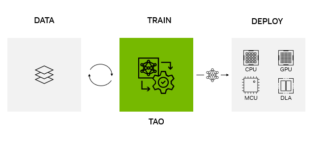
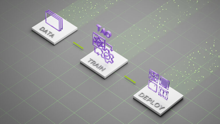
Graphic of the NVIDIA TAO Toolkit pipeline for an AI model: data, train, and deploy.
Figure 1. NVIDIA TAO Toolkit workflow diagram

Deploy NVIDIA TAO models on any platform, anywhere 

NVIDIA TAO Toolkit 5.0 supports model export in ONNX. This makes it possible to deploy a model trained with NVIDIA TAO Toolkit on any computing platform—GPUs, CPUs, MCUs, DLAs, FPGAs—at the edge or in the cloud. NVIDIA TAO Toolkit simplifies the model training process and optimizes the model for inference throughput, powering AI across hundreds of billions of devices.  
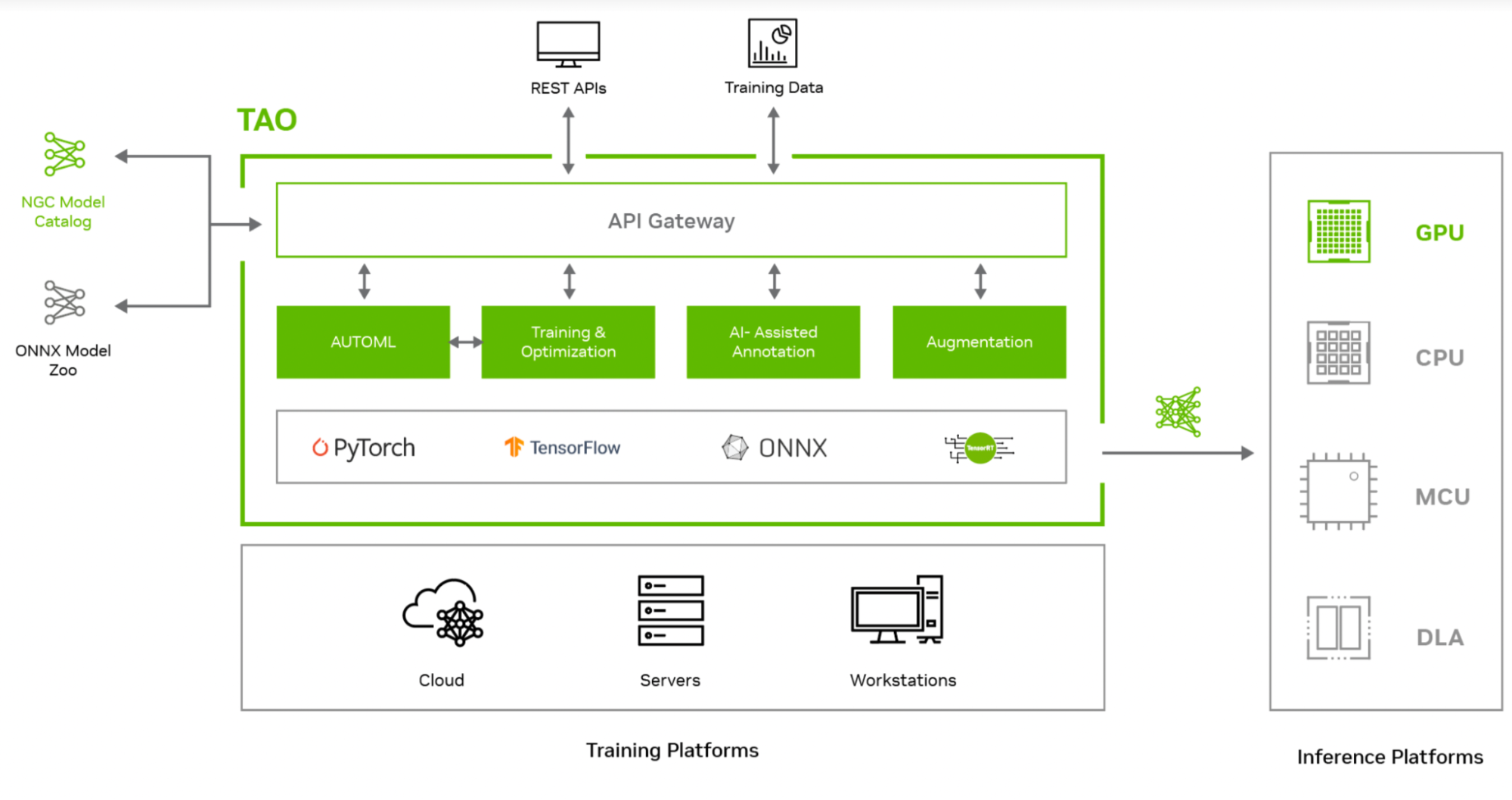
TAO Toolkit architecture workflow diagram.
Figure 2. NVIDIA TAO Toolkit architecture

Edge Impulse, a platform for building, refining, and deploying machine learning models and algorithms, integrated TAO Toolkit into their edge AI platform. With this integration, Edge Impulse now offers advanced vision AI capabilities and models that complement its current offerings. Developers can use the platform to build production AI with TAO for any edge device. Learn more about the integration in a blog post from Edge Impulse.

Video 1. Training an AI model with the Edge Impulse platform leveraging NVIDIA TAO and deployed on a Cortex-M7 MCU

STMicroelectronics, a global leader in embedded microcontrollers, integrated NVIDIA TAO Toolkit into its STM32Cube AI developer workflow. This puts the latest AI capabilities into the hands of millions of STMicroelectronics developers. It provides, for the first time, the ability to integrate sophisticated AI into widespread IoT and edge use cases powered by the STM32Cube. 

Now, with NVIDIA TAO Toolkit, even the most novice AI developers can optimize and quantize AI models to run on STM32 MCU within the microcontroller’s compute and memory budget. Developers can also bring their own models and fine-tune using TAO Toolkit. More information about this work is captured in the following demo. Learn more about the project on the STMicroelectronics GitHub page.

Video 2. Learn how to deploy a model optimized with TAO Toolkit on an STM microcontroller

While TAO Toolkit models can run on any platform, these models achieve the highest throughput on NVIDIA GPUs using TensorRT for inference. On CPUs, these models use ONNX-RT for inference. The script and recipe to replicate these numbers will be provided once the software becomes available.

  NVIDIA Jetson Orin Nano 8 GB  NVIDIA Jetson AGX Orin 64 GB  T4  A2  A100 L4  H100  
PeopleNet  112  679 429 242 3,264 797 7,062
DINO – FAN-S  3.1 11.2 20.4 11.7 121 44 213
SegFormer – MiT 1.3 4.8  9.4 5.8 62.2 17.8 108
OCRNet  935  3,876 3,649 2,094 28,300 8,036 55,700
EfficientDet  61 227 303 184 1,521 522 2,428
2D Body Pose  136  557 593 295 4,140 1,010 7,812
3D Action Recognition  52 212 269 148 1,658 529 2,708
Table 1. Performance comparison (in FPS) of several NVIDIA TAO Toolkit vision models, including new Vision Transformer models on NVIDIA GPUs

AI-assisted data annotation and management 

Data annotation remains an expensive and time-consuming process for all AI projects. This is especially true for CV tasks like segmentation that require generating a segmentation mask at pixel level around the object. Generally, segmentation masks cost 10x more than object detection or classification. 

It is faster and less expensive to annotate segmentation masks with new AI-assisted annotation capabilities using TAO Toolkit 5.0. Now you can use the weakly supervised segmentation architecture, Mask Auto Labeler (MAL) to aid in segmentation annotation and in fixing and tightening bounding boxes for object detection. Loose bounding boxes around an object in ground truth data can lead to suboptimal detection results. But, with AI-assisted annotation, you can tighten your bounding boxes over objects, leading to more accurate models.  

GIF showing the concept of auto-labeling of cars and a person holding a grocery basket, using box-cropped images as inputs, and generating the segmentation mask.
Figure 3. TAO Toolkit auto labeling

MAL is a transformer-based, mask auto-labeling framework for instance segmentation using only box annotations. MAL takes box-cropped images as inputs and conditionally generates the mask pseudo-labels. It uses COCO annotation format for both input and output labels.  

MAL significantly reduces the gap between auto labeling and human annotation for mask quality. Instance segmentation models trained using the MAL-generated masks can nearly match the performance of the fully supervised counterparts, retaining up to 97.4% performance of fully supervised models.  
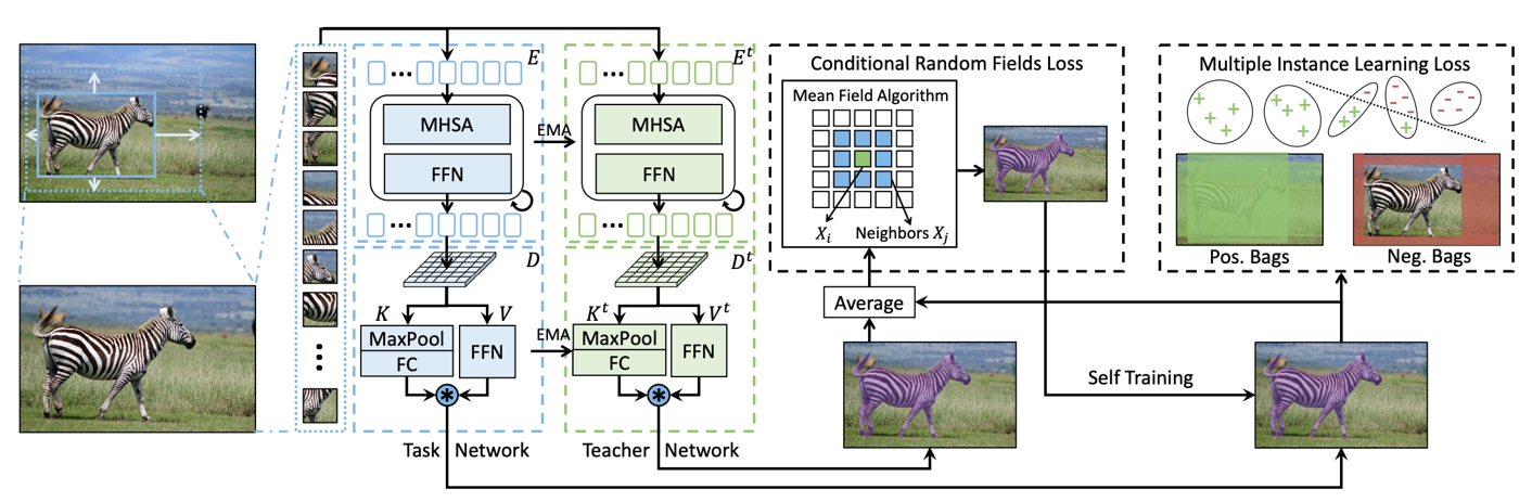
Architecture diagram for Mask Auto Labeler (MAL).
Figure 4. MAL network architecture

When training the MAL network, a task network and a teacher network (sharing the same transformer structure) work together to achieve class-agnostic self-training. This enables refining the prediction masks with conditional random field (CRF) loss and multi-instance learning (MIL) loss.    

TAO Toolkit uses MAL in both the auto-labeling pipeline and data augmentation pipeline. Specifically, users can generate pseudo-masks on the spatially augmented images (sheared or rotated, for example), and refine and tighten the corresponding bounding boxes using the generated masks. 

State-of-the-art Vision Transformers 

Transformers have become the standard architecture in NLP, largely because of self-attention. They have also gained popularity for a range of vision AI tasks. In general, transformer-based models can outperform traditional CNN-based models due to their robustness, generalizability, and ability to perform parallelized processing of large-scale inputs. All of this increases training efficiency, provides better robustness against image corruption and noise, and generalizes better on unseen objects.  

TAO Toolkit 5.0 features several state-of-the-art (SOTA) Vision Transformers for popular CV tasks, as detailed below.

Fully Attentional Network  

Fully Attentional Network (FAN) is a transformer-based family of backbones from NVIDIA Research that achieves SOTA in robustness against various corruptions. This family of backbones can easily generalize to new domains and be more robust to noise, blur, and more. 

A key design behind the FAN block is the attentional channel processing module that leads to robust representation learning. FAN can be used for image classification tasks as well as downstream tasks such as object detection and segmentation.  

Performing heat map on a corrupted image (left) using ResNet50 (center) and FAN-Small (right).
Figure 5. An activation heat map on a corrupted image for ResNet50 (center) compared to FAN-Small (right)

The FAN family supports four backbones, as shown in Table 2.

Model  # of parameters/FLOPs  Accuracy 
FAN-Tiny  7 M/3.5 G  71.7 
FAN-Small  26 M/6.7  77.5 
FAN-Base  50 M/11.3 G  79.1 
FAN-Large  77 M/16.9 G  81.0 
Table 2. FAN backbones with size and accuracy

Global Context Vision Transformer 

Global Context Vision Transformer (GC-ViT) is a novel architecture from NVIDIA Research that achieves very high accuracy and compute efficiency. GC-ViT addresses the lack of inductive bias in Vision Transformers. It achieves better results on ImageNet with a smaller number of parameters through the use of local self-attention. 

Local self-attention paired with global context self-attention can effectively and efficiently model both long and short-range spatial interactions. Figure 6 shows the GC-ViT model architecture. For more details, see Global Context Vision Transformers.

Diagram of the architecture for GC-ViT.
Figure 6. GC-ViT model architecture

As shown in Table 3, the GC-ViT family contains six backbones, ranging from GC-ViT-xxTiny (compute efficient) to GC-ViT-Large (very accurate). GC-ViT-Large models can achieve Top-1 accuracy of 85.6 on the ImageNet-1K dataset for image classification tasks. This architecture can also be used as the backbone for other CV tasks like object detection and semantic and instance segmentation.  

Model  # of parameters/FLOPs  Accuracy 
GC-ViT-xxTiny  12 M/2.1 G  79.6 
GC-ViT-xTiny  20 M/2.6 G  81.9 
GC-ViT-Tiny  28 M/4.7 G  83.2 
GC-ViT-Small  51 M/8.5 G  83.9 
GC-ViT-Base  90 M/14.8 G  84.4 
GC-ViT-Large  201 M/32.6 G  85.6 
Table 3. GC-ViT backbones with size and accuracy 

DINO 

DINO (detection transformer with improved denoising anchor) is the newest generation of detection transformers (DETR). It achieves a faster training convergence time than its predecessor. Deformable-DETR (D-DETR) requires at least 50 epochs to converge, while DINO can converge in 12 epochs on the COCO dataset. It also achieves higher accuracy when compared with D-DETR. 

DINO achieves faster convergence through the use of denoising during training, which helps the bipartite matching process at the proposal generation stage. The training convergence of DETR-like models is slow due to the instability of bipartite matching. Bipartite matching removed the need for handcrafted and compute-heavy NMS operations. However, it often required much more training because incorrect ground truths were matched to the predictions during bipartite matching. 

To remedy such a problem, DINO introduced noised positive ground-truth boxes and negative ground-truth boxes to handle “no object” scenarios. As a result, training converges very quickly for DINO. For more information, see DINO: DETR with Improved DeNoising Anchor Boxes for End-to-End Object Detection.
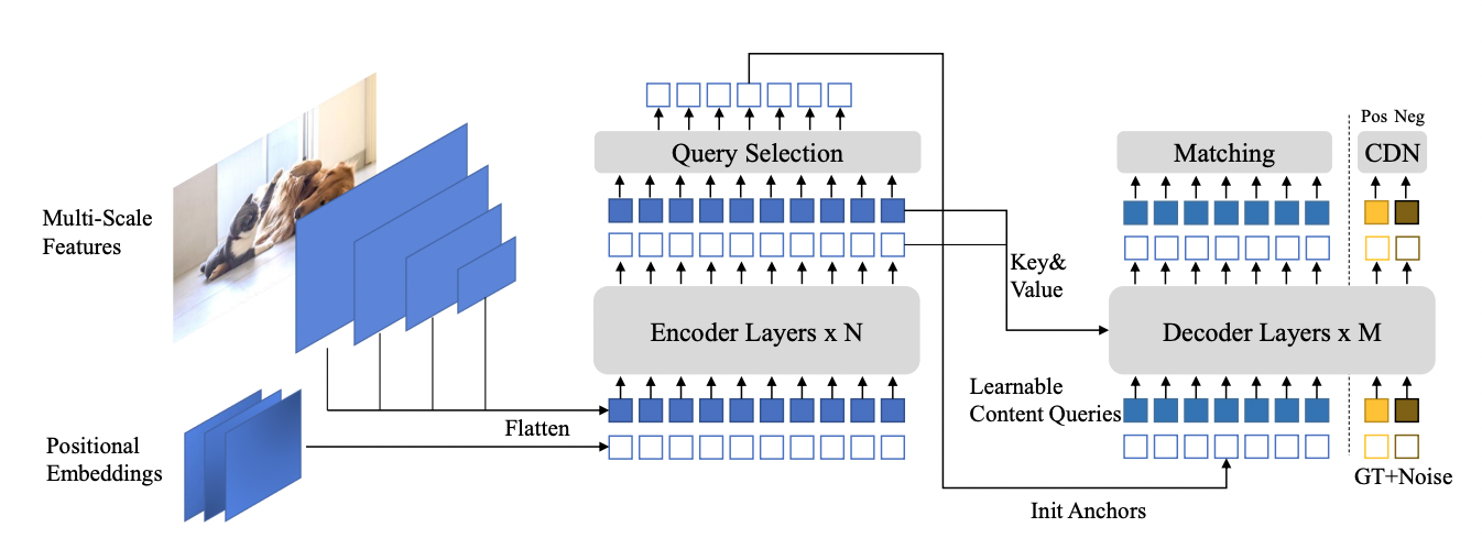
Diagram of DINO architecture, including multi-scale features, positional embeddings, query selection, encoder layers, matching, CDN, and decoder layers.
Figure 7. DINO architecture

DINO in TAO Toolkit is flexible and can be combined with various backbones from traditional CNNs, such as ResNets, and transformer-based backbones like FAN and GC-ViT. Table 4 shows the accuracy of the COCO dataset on various versions of DINO with popular YOLOv7. For more details, see YOLOv7: Trainable Bag-of-Freebies Sets New State-of-the-Art for Real-Time Object Detectors.

Model Backbone AP AP50 AP75 APS APM APL Param
YOLOv7 N/A 51.2 69.7 55.5 35.2 56.0 66.7 36.9M
DINO ResNet50 48.8 66.9 53.4 31.8 51.8 63.4 46.7M
FAN-Small 53.1 71.6 57.8 35.2 56.4 68.9 48.3M
GCViT-Tiny 50.7 68.9 55.3 33.2 54.1 65.8 46.9M
Table 4. DINO and D-DETR accuracy on the COCO dataset

SegFormer 

SegFormer is a lightweight transformer-based semantic segmentation. The decoder is made of lightweight MLP layers. It avoids using positional encoding (mostly used by transformers), which makes the inference efficient at different resolutions.  

Adding FAN backbone to SegFormer MLP decoder results in a highly robust and efficient semantic segmentation model. FAN base hybrid + SegFormer was the winning architecture at the Robust Vision Challenge 2022 for semantic segmentation. 
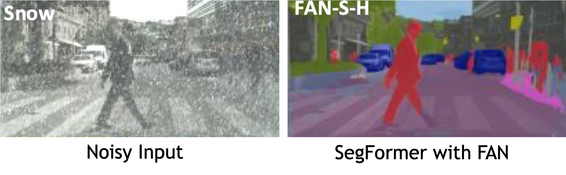
An image of a man walking across the street as a noisy input (left) and the same image with SegFormer with FAN (right).
Figure 8. SegFormer with FAN prediction (right) on a noisy input image (left) 
Model   Dataset  Mean IOU (%)  Retention rate (robustness) (%) 
PSPNet  Cityscapes Validation  78.8  43.8  
SegFormer – FAN-S-Hybrid  Cityscapes validation  81.5  81.5 
Table 5. Robustness of SegFormer compared to PSPNet

See how SegFormer generates robust semantic segmentation while maintaining high efficiency for accelerated autonomous vehicle development in the following video. 

Video 3. NVIDIA DRIVE Labs episode, Enhancing AI Segmentation Models for Autonomous Vehicle Safety

CV tasks beyond object detection and segmentation 

NVIDIA TAO Toolkit accelerates a wide range of CV tasks beyond traditional object detection and segmentation. The new character detection and recognition models in TAO Toolkit 5.0 enable developers to extract text from images and documents. This automates document conversion and accelerates use cases in industries like insurance and finance.  

Detecting anomalies in images is useful when the object being classified varies greatly, such that training with all the variations is impossible. In industrial inspection, for example, a defect can come in any form. Using a simple classifier could result in many missed defects if the defect has not been previously seen by the training data. 

For such use cases, comparing the test object directly against a golden reference would result in better accuracy. TAO Toolkit 5.0 features a Siamese neural network in which the model calculates the difference between the object under test and a golden reference to classify if the object is defective.  

Automate training using AutoML for hyperparameter optimization 

Automated machine learning (autoML) automates the manual task of finding the best models and hyperparameters for the desired KPI on a given dataset. It can algorithmically derive the best model and abstract away much of the complexity of AI model creation and optimization.  

AutoML in TAO Toolkit is fully configurable for automatically optimizing the hyperparameters of a model. It caters to both AI experts and nonexperts. For nonexperts, the guided Jupyter Notebook provides a simple, efficient way to create an accurate AI model. 

For experts, TAO Toolkit gives you full control of which hyperparameters to tune and which algorithm to use for sweeps. TAO Toolkit currently supports two optimization algorithms: Bayesian and Hyperband optimization. These algorithms can sweep across a range of hyperparameters to find the best combination for a given dataset. 

AutoML is supported for a wide range of CV tasks, including several new Vision Transformers such as DINO, D-DETR, SegFormer, and more. Table 6 shows the full list of supported networks (bold items are new to TAO Toolkit 5.0). 

Image classification Object detection Segmentation Other
FAN DINO SegFormer LPRNet
GC-ViT D-DETR UNET
ResNet YoloV3/V4/V4-Tiny MaskRCNN
EfficientNet EfficientDet 
DarkNet RetinaNet
MobileNet FasterRCNN
DetectNet_v2
SSD/DSSD
Table 6. Models supported by AutoML in TAO Toolkit, including several new Vision Transformer models (bold items are new to TAO Toolkit 5.0)

REST APIs for workflow integration 

TAO Toolkit is modular and cloud-native, meaning it is available as containers and can be deployed and managed using Kubernetes. TAO Toolkit can be deployed as a self-managed service on any public or private cloud, DGX, or workstation. TAO Toolkit provides well-defined REST APIs, making it easy to integrate into your development workflow. Developers can call the API endpoints for all training and optimization tasks. These API endpoints can be called from any application or user interface, which can trigger training jobs remotely. 
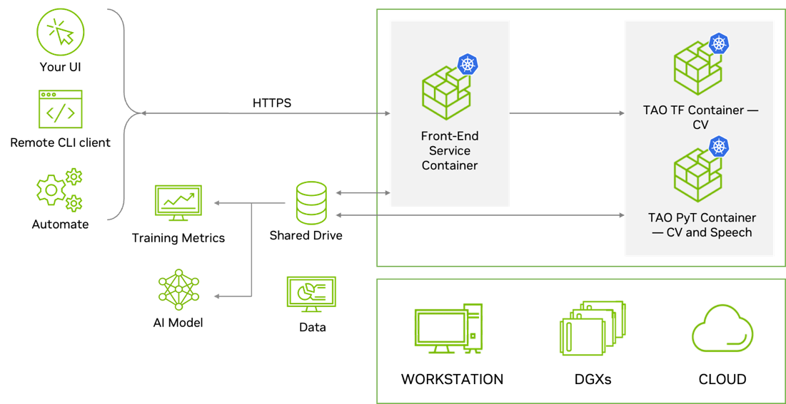
REST APIs workflow in TAO Toolkit
Figure 9. TAO Toolkit architecture for cloud native deployment

Better inference optimization 

To simplify productization and increase inference throughput, TAO Toolkit provides several turnkey performance optimization techniques. These include model pruning, lower precision quantization, and TensorRT optimization, which can combine to deliver a 4x to 8x performance boost, compared to a comparable model from public model zoos. 
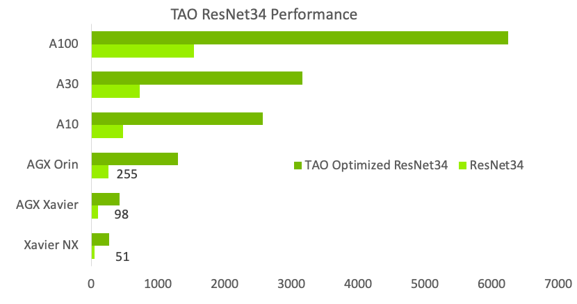
Chart showing performance comparison between TAO Toolkit optimized and public models on a wide range of GPUs
Figure 10. Performance comparison between TAO Toolkit optimized and public models on a wide range of GPUs

Open and flexible, with better support 

An AI model predicts output based on complex algorithms. This can make it difficult to understand how the system arrived at its decision and challenging to debug, diagnose, and fix errors. Explainable AI (XAI) aims to address these challenges by providing insights into how AI models arrive at their decisions. This helps humans understand the reasoning behind the AI output and makes it easier to diagnose and fix errors. This transparency can help to build trust in AI systems. 

To help with transparency and explainability, TAO Toolkit will now be available as source-open. Developers will be able to view feature maps from internal layers, as well as plot activation heat maps to better understand the reasoning behind AI predictions. In addition, having access to the source code will give developers the flexibility to create customized AI, improve debug capability, and increase trust in their models.  

NVIDIA TAO Toolkit is enterprise-ready and available through NVIDIA AI Enterprise (NVAIE). NVAIE provides companies with business-critical support, access to NVIDIA AI experts, and priority security fixes. Join NVAIE to get support from AI experts.  

Integration with cloud services 

NVIDIA TAO Toolkit 5.0 is integrated into various AI services that you might already use, such as Google Vertex AI, AzureML, Azure Kubernetes service, Google GKE, and Amazon EKS. 
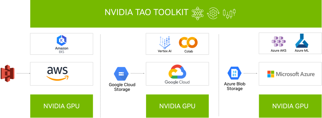
Graphic showing the TAO framework for various cloud services, including Google Cloud, Microsoft Azure, and more.
Figure 11. TAO Toolkit 5.0 is integrated with various AI services

Summary 

TAO Toolkit offers a platform for any developer, in any service, and on any device to easily transfer-learn their custom models, perform quantization and pruning, manage complex training workflows, and perform AI-assisted annotation with no coding requirements.

Categories
Misc

Fin-tastic: 3D Artist Dives Into AI-Powered Oceanic Work This Week ‘In the NVIDIA Studio’

We’re gonna need a bigger boat this week In the NVIDIA Studio as Alessandro Mastronardi, senior artist and programmer at BBC Studios, shares heart-stopping shark videos and renders.

Categories
Misc

NVIDIA DGX Cloud Now Available to Supercharge Generative AI Training

NVIDIA DGX Cloud — which delivers tools that can turn nearly any company into an AI company —  is now broadly available, with thousands of NVIDIA GPUs online on Oracle Cloud Infrastructure, as well as NVIDIA infrastructure located in the U.S. and U.K. Unveiled at NVIDIA’s GTC conference in March, DGX Cloud is an AI Read article >

Categories
Misc

NVIDIA Names Melissa Lora to Board of Directors

SANTA CLARA, Calif., July 24, 2023 (GLOBE NEWSWIRE) — NVIDIA today announced that it has named to its board of directors Melissa Lora, who spent three decades as an executive at Taco Bell …

Categories
Misc

Realizing the Power of Real-Time Network Processing with NVIDIA DOCA GPUNetIO

Real-time processing of network traffic can be leveraged by the high degree of parallelism GPUs offer. Optimizing packet acquisition or transmission in these…
Real-time processing of network traffic can be leveraged by the high degree of parallelism GPUs offer. Optimizing packet acquisition or transmission in these types of applications avoids bottlenecks and enables the overall execution to keep up with high-speed networks. In this context, DOCA GPUNetIO promotes the GPU as an independent component that can exercise network and compute tasks without the intervention of the CPU.

This post provides a list of GPU packet processing applications focusing on different and unrelated contexts where NVIDIA DOCA GPUNetIO has been integrated to lower latency and maximize performance.

NVIDIA DOCA GPUNetIO API

NVIDIA DOCA GPUNetIO is one of the new libraries released with the NVIDIA DOCA software framework. The DOCA GPUNetIO library enables direct communication between the NIC and the GPU through one or more CUDA kernels. This removes the CPU from the critical path. 

Using the CUDA device functions in the DOCA GPUNetIO library, a CUDA kernel can send and receive packets directly from and to the GPU without the need of CPU cores or memory. Key features of this library include:

  • GPUDirect Async Kernel-Initiated Network (GDAKIN): Communications over Ethernet; GPU (CUDA kernel) can directly interact with the network card to send or receive packets in GPU memory (GPUDirect RDMA) without the intervention of the CPU.
  • GPU memory exposure: Combine within a single function the basic CUDA memory allocation feature with the GDRCopy library to expose a GPU memory buffer to the direct access (read or write) from the CPU without using CUDA API.
  • Accurate Send Scheduling: From the GPU, it’s possible to schedule the transmission of a burst of packets in the future, associate a timestamp to it, and provide this information to the network card, which will in turn take care of sending packets at the right time.
  • Semaphores: Useful message passing object to share information and synchronize across different CUDA kernels or between a CUDA kernel and a CPU thread.

For a deep dive into the principles and benefits of DOCA GPUNetIO, see Inline GPU Packet Processing with NVIDIA DOCA GPUNetIO. For more details about DOCA GPUNetIO API, refer to the DOCA GPUNetIO SDK Programming Guide.

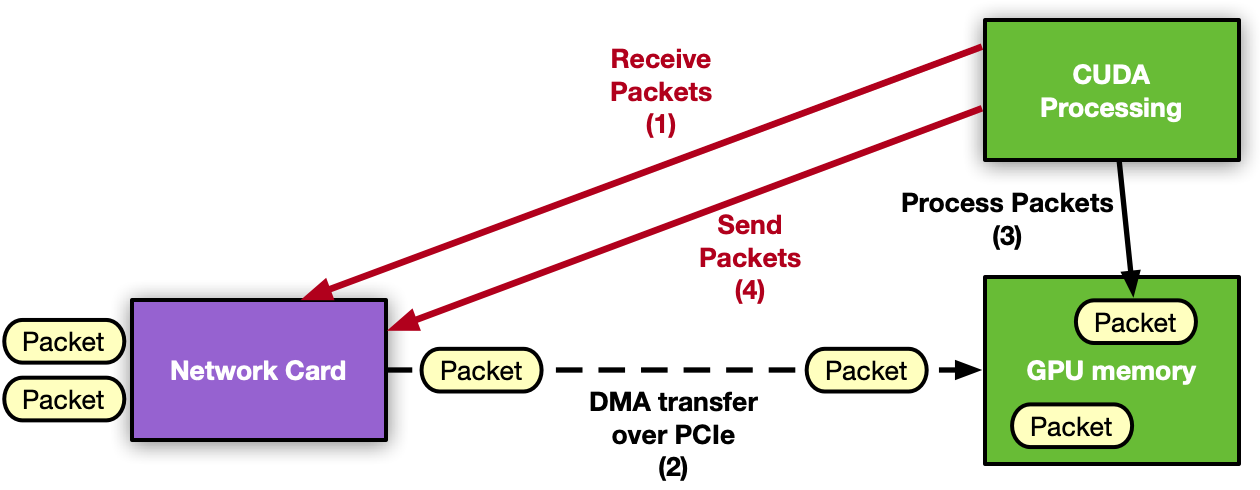
Diagram showing a GPU-centric application in which the GPU can execute both network tasks (receive and send) and processing tasks. The CPU is no longer required.
Figure 1. Layout of the receive process in an NVIDIA DOCA GPUNetIO application. No CPU is involved, as the GPU can independently receive and process network packets

Along with the library, the following NVIDIA DOCA application and NVIDIA DOCA sample show how to use functions and features offered by the library. 

  • NVIDIA DOCA application: A GPU packet processing application that can detect, manage, filter, and analyze UDP, TCP, and ICMP traffic. The application also implements an HTTP over TCP server. With a simple HTTP client (curl or wget, for example), it’s possible to establish a TCP three-way handshake connection and ask for simple HTML pages through HTTP GET requests to the GPU.
  • NVIDIA DOCA sample: GPU send-only example that shows how to use the Accurate Send Scheduling feature (system configuration, functions to use).

DOCA GPUNetIO in real-world applications

DOCA GPUNetIO has been used to empower the NVIDIA Aerial SDK to send and receive using the GPU, getting rid of the CPU. For more details, see Inline GPU Packet Processing with NVIDIA DOCA GPUNetIO. The sections below provide new examples that successfully use DOCA GPUNetIO to leverage the GPU packet acquisition with the GDAKIN technique.

NVIDIA Morpheus AI

NVIDIA Morpheus is a performance-oriented, application framework that enables cybersecurity developers to create fully optimized AI pipelines for filtering, processing, and classifying large volumes of real-time data. The framework abstracts GPU and CPU parallelism and concurrency through an accessible programming model consisting of Python and C++ APIs. 

Leveraging this framework, developers can quickly construct arbitrary data pipelines composed of stages that acquire, mutate, or publish data for a downstream consumer. You can apply Morpheus in different contexts including malware detection, phishing/spear phishing detection, ransomware detection, and many others. Its flexibility and high performance are ideal for real-time network traffic analysis.

For the network monitoring use case, the NVIDIA Morpheus team recently integrated the DOCA framework to implement a high-speed, low-latency GPU packet acquisition source stage to feed real-time packets to an AI-pipeline responsible for analyzing packets’ contents. For more details, visit Morpheus on GitHub.

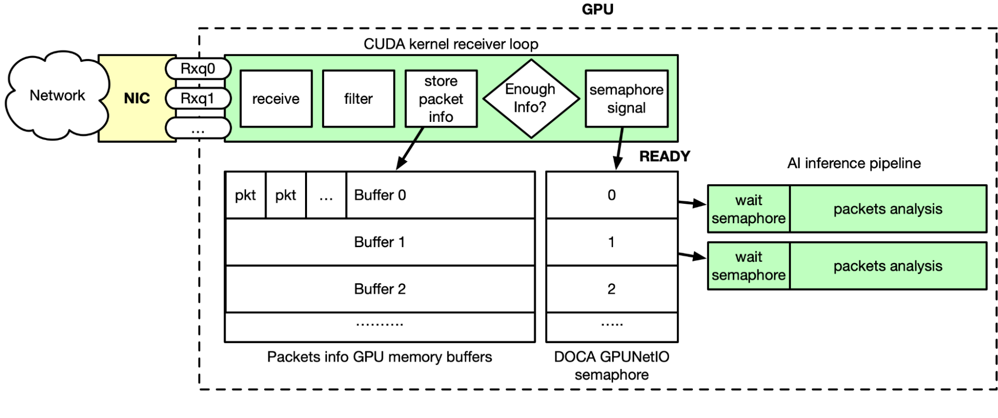
A diagram showing the point of connection between DOCA GPUNetIO and Morpheus AI pipeline. If the packets pass the filter, their information is stored in a GPU memory buffer, accumulate, and trigger AI processing.
Figure 2. DOCA GPUNetIO and NVIDIA Morpheus AI pipeline are connected by a CUDA kernel that receives, filters, and analyzes incoming packets

As shown in Figure 2, GPU packet acquisition happens in real time. Through DOCA Flow, flow steering rules are applied to the Ethernet receive queues, meaning queues can only receive specific types of packets (TCP, for example). Morpheus launches a CUDA kernel, which performs the following steps in a loop:

  1. Receive packets using DOCA GPUNetIO receive function
  2. Filter and analyze in parallel packets in GPU memory
  3. Copy relevant packets info in a list of GPU memory buffers
  4. The related DOCA GPUNetIO semaphore item is set to READY when a buffer has accumulated enough packets of information
  5. The CUDA kernel in front of the AI pipeline is polling the semaphore item
  6. When the item is READY, AI is unblocked as packet information is ready in the buffer

The GTC session Defensive Cyber Operations (DCO) on Edge Networks presents a concrete example in which this architecture is leveraged to deploy a high-performance, AI-enabled SPAN/Network TAP solution. This solution was motivated by the daunting data rates in information technology (IT) and operational technology (OT) networks, heterogeneity of Layer 7 application data, and edge computing size, weight, and power (SWaP) constraints. 

In the case of edge computing, many organizations are unable to “burst to cloud” when the compute demand increases, especially on disconnected edge networks. This scenario requires designing an architecture for I/O and compute challenges that deliver performance across the SWaP spectrum.

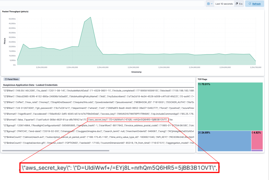
This DCO example addresses these constraints through the lens of a common cybersecurity problem, identifying leaked data (leaked passwords, secret keys, and PII, for example) in unencrypted TCP traffic, and represents an extension of the Morpheus SID demo. Identifying and remediating these vulnerabilities reduces the attack surface and increases the security posture of organizations.

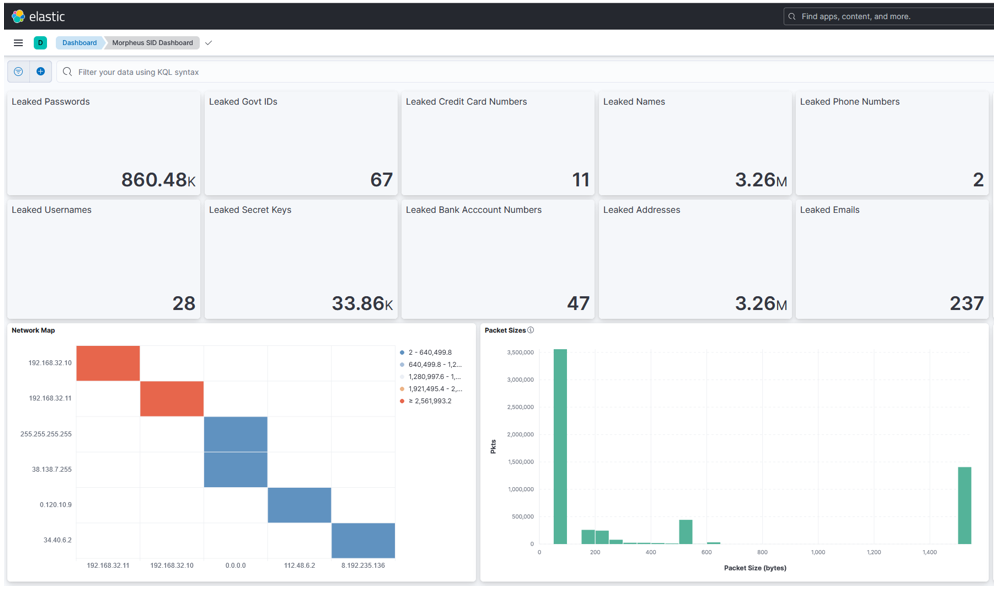
In this example, the DCO solution receives packets into a heterogeneous Morpheus pipeline (GPU and concurrent CPU stages written in a mix of Python and C++) that applies a transformer model to detect leaked sensitive data in Layer 7 application data. It integrates outputs with the ELK stack, including an intuitive visualization for Security Operations Center (SOC) analysts to exploit (Figures 3 and 4).

Example Kibana dashboard showcasing results of DOCA GPUNetIO plus Morpheus Sensitive Information Detections including total detections of each type, a pairwise network map, and the distribution of packet sizes.
Figure 3. Kibana dashboard showcasing results of DOCA GPUNetIO plus Morpheus Sensitive Information Detections including total detections of each type, a pairwise network map, and the distribution of packet sizes
Screenshot of Kibana dashboard showcasing results of DOCA GPUNetIO plus Morpheus Sensitive Information Detections including filtered and processed network packets index at up to 50 K packets per second, including a table of payloads with leaked secret keys.
Figure 4. Kibana dashboard showcasing results of DOCA GPUNetIO plus Morpheus Sensitive Information Detections including filtered and processed network packets index at up to 50 K packets per second, including a table of payloads with leaked secret keys

The experimental setup included cloud-native UDP multicast and REST applications running on VMs with a 100 Gbps NVIDIA BlueField-2 DPU. These applications communicated through a SWaP-efficient NVIDIA Spectrum SN2100 Ethernet switch. Packet generators injected sensitive data into packets transmitted by these applications. Network packets were aggregated and mirrored off a SPAN port on the NVIDIA Spectrum SN2100 and sent to an NVIDIA A30X converged accelerator powering the Morpheus packet inspection pipeline achieving impressive throughput results.

  • This pipeline includes several components from I/O, packet filtering, packet processing, and indexing in a third-party SIEM platform (Elasticsearch). Focusing only on the I/O aspects, DOCA GPUNetIO enables Morpheus to receive packets into GPU memory at up to 100 Gbps with a single receive queue, removing a critical bottleneck in cyber packet processing applications.
  • Leveraging stage level concurrency, the pipeline demonstrated a 60% boost in Elasticsearch indexing throughput.
  • Running the end-to-end data pipeline on the NVIDIA A30X converged accelerator generated enriched packets at ~50% capacity of the elasticsearch indexer. Using twice as many A30Xs would fully saturate the indexer, providing a convenient scaling heuristic.
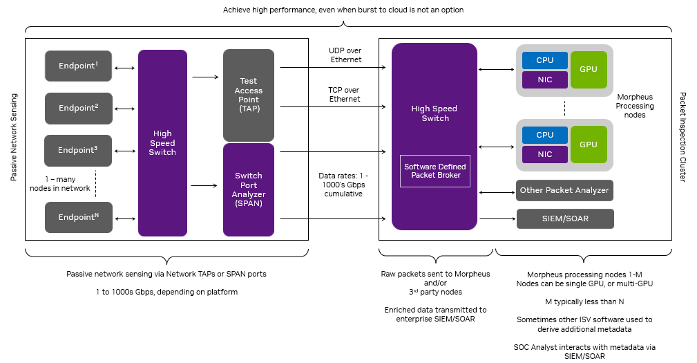
This figure depicts the end-to-end accelerated sensitive information detection packet processing application. SOC teams who leverage other SIEM/SOAR solutions (such as Splunk) are empowered to exchange Morpheus sink stages in their implementations.
Figure 5. The end-to-end packet processing application accelerates the detection of sensitive information

While this use case demonstrates a specific application of Morpheus, it represents the foundational components for cyber packet processing applications. Morpheus plus DOCA GPUNetIO together provide the performance and extensibility for a huge number of latency-sensitive and compute-intensive packet processing applications.

Line-rate radar signal processing

This section walks through an example in which the radar detection application ingests downconverted I/Q samples from a simulated range-only radar system at line rate of 100 Gbps, performing all required signal processing needed to convert the received I/Q RF samples into object detections in real time.

Remote sensing applications such as radar, lidar, and optical platforms rely on signal processing algorithms to turn the raw data collected from the environment they are measuring into actionable information. These algorithms are often highly parallelizable and require a high computational load, making them ideal for GPU-based processing.

Additionally, input sensors generate enormous quantities of raw data, meaning the ingress/egress capability of the processing solution must be able to handle very high bandwidths at low latencies. 

Further complicating the problem, many edge-based sensor systems have strict SWaP constraints, restricting the number and power of available CPU cores that might be used in other high-throughput networking approaches, such as DPDK-based GPUDirect RDMA.

DOCA GPUNetIO enables the GPU to directly handle the networking load as well as the signal processing required to make a real-time sensor streaming application successful.

Commonly used signal processing algorithms were used in the radar detection application. The flowchart in Figure 6 shows a graphical representation of the signal processing pipeline being used to convert the I/Q samples into detections.

Flowchart depicting the building blocks of a signal processing pipeline for computing detections from a reflected RF waveform in a range-only radar system. Stages are MTI Filtering, Pulse compression with FFR and Inverse FFT, and finally CFAR Detection.
Figure 6. The signal processing pipeline for computing detections from a reflected RF waveform in a range-only radar system

MTI filtering is a common technique used to eliminate stationary background clutter, such as the ground or buildings, from the reflected RF waveform in radar systems. The approach used here is known as the Three-Pulse Canceler, which is simply a convolution of the I/Q data in the pulse dimension with the filter coefficients ‘[+1, -2, +1].’

Pulse Compression maximizes the signal-to-noise ratio (SNR) of the received waveform with respect to the presence of targets. It is performed by computing the cross-correlation of the received RF data with the transmitted waveform.

Constant False Alarm Rate (CFAR) detectors compute an empirical estimate of the noise, localized to each range bin of the filtered data. The power of each bin is then compared to the noise and declared a detection if it is statistically likely given the noise estimate and distribution.

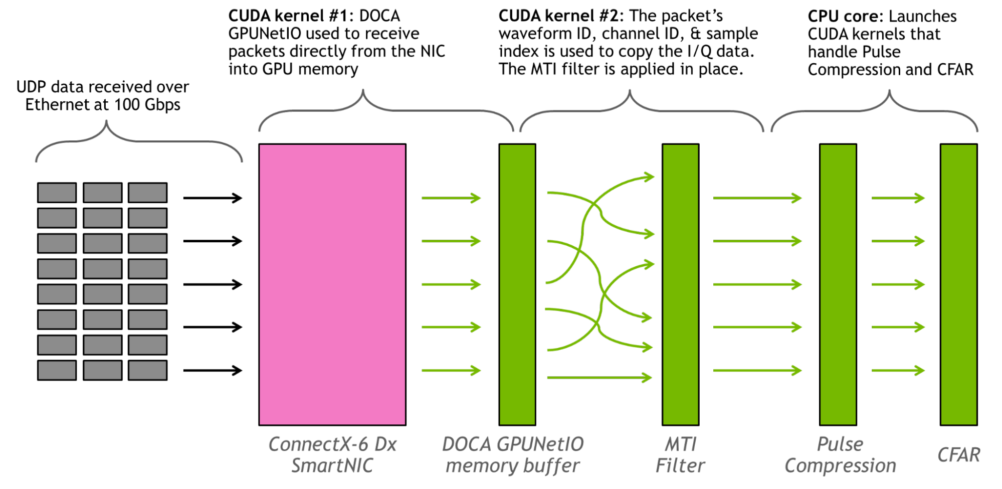
A 3D buffer of size (# Waveforms) x (# Channels) x (# Samples) is used to hold the organized RF data being received (note that applying the MTI filter upon packet receipt reduces the size of the pulse dimension to 1). No ordering is assumed to the UDP data streaming in, except that it is streamed roughly in order of the packets’ ascending waveform ID. Around 500 complex samples are transmitted per-packet, and the samples’ location in the 3D buffer is dependent on the waveform ID, channel ID, and sample index.

This application runs two CUDA kernels and one CPU core persistently. The first CUDA kernel is responsible for using the DOCA GPUNetIO API to read packets from the NIC onto the GPU. The second CUDA kernel places packet data into the correct memory location based on metadata in the packets header and applies the MTI filter, and the CPU core is responsible for launching the CUDA kernels that handle Pulse Compression and CFAR. The FFTs were performed using the cuFFT library.

Figure 7 shows a graphical representation of the application.

Figure depicts the GPU-based signal processing pipeline with two CUDA kernels: one using DOCA GPUNetIO to receive packets in GPU memory and a second to analyze packets.
Figure 7. Graphical representation of how work is distributed for the GPU-based signal processing pipeline

The throughput of the radar detection pipeline is >100 Gbps. Running at the line rate of 100 Gbps for 1 million 16-channel waveforms, no packets were dropped and the signal processing never fell behind the throughput of the data stream. The latency, measured from when the last data packet for an independent waveform ID was received, was on the order of 3 milliseconds. An NVIDIA ConnectX-6 Dx SmartNIC and an NVIDIA A100 80 GB GPU were used. Data was sent through UDP packets over Ethernet.

Future work will evaluate the performance of this architecture when running exclusively on a BlueField DPU with an integrated GPU.

Real-time DSP services over GPU

Analog signals are everywhere, both artificial (Wi-Fi radio, for example) and natural (solar radiation and earthquakes, for example). To capture analog data digitally, sound waves must be converted using a D-A converter, controlled by parameters such as sample rate and sample bit depth. Digital audio and video can be processed with FFT, allowing sound designers to use tools such as an equalizer (EQ) to alter general characteristics of the signal.

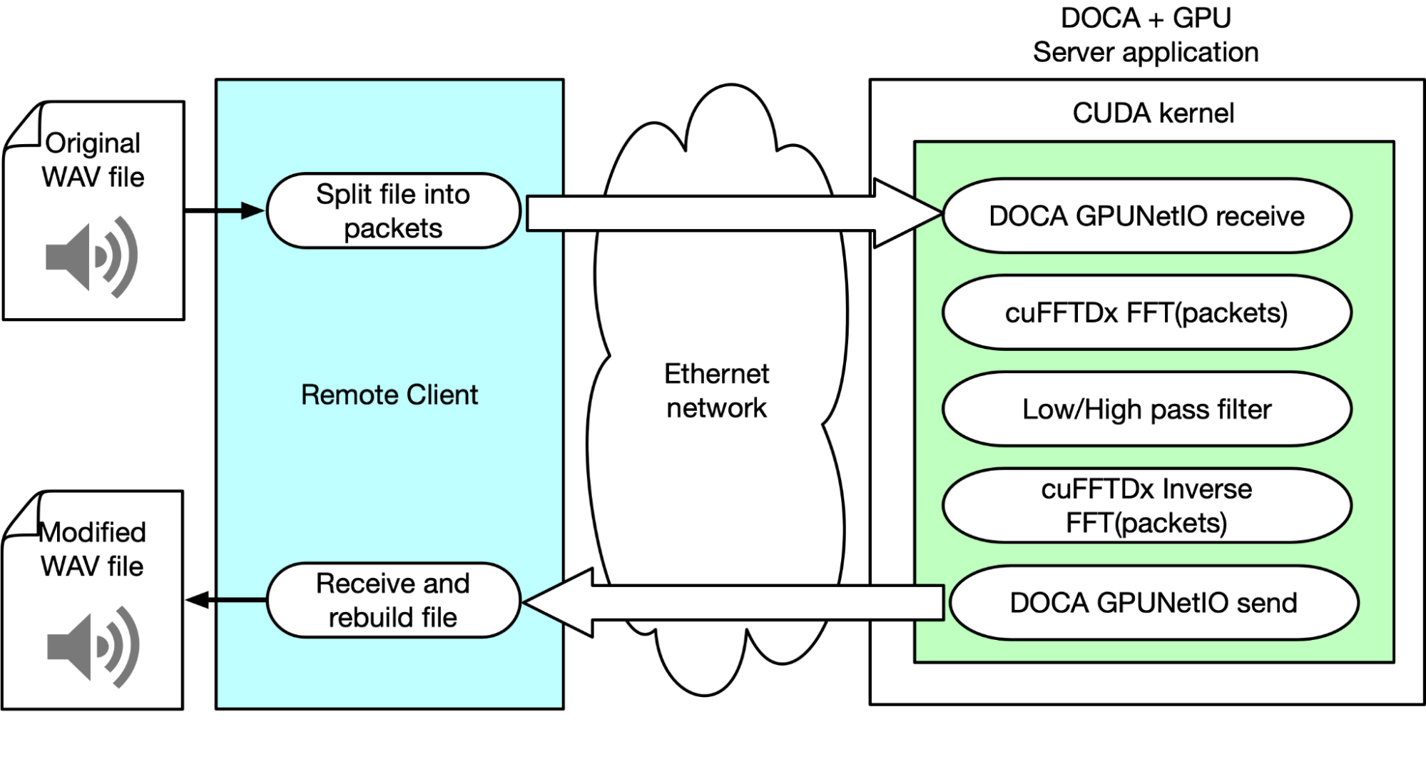
This example explains how NVIDIA products and SDK were used to perform real-time audio DSP with GPU over the network. To do so, the team built a client that parses a WAV file, frames data into multiple Ethernet packets, and sends them over the network to a server application. This application is responsible for receiving packets, applying FFT, manipulating the audio signal, and finally sending back the modified data.

The client’s responsibility is recognizing which portion should be sent to the “server” for the signal processing chain and how to treat the processed samples when they are received back from the server. This approach supports multiple DSP algorithms, such as overlap-add, and various sample window selections.

The server application uses DOCA GPUNetIO to receive packets in GPU memory from a CUDA kernel. When a subset of packets has been received, the CUDA kernel in parallel applies the FFT through the cuFFTDx library to each packet’s payload. In parallel, to each packet, a different CUDA thread applies a frequency filter reducing the amplitude of low or high frequencies. Basically, it applies a low-pass or high-pass filter.

Diagram depicting the client-server architecture where the client splits a WAV file into multiple Ethernet packets and sends them to the server. On the server, a CUDA kernel in a continuous loop receives those packets, applies frequency filters and then sends back the modified packets.
Figure 8. Client-server architecture built to demonstrate how to do real-time DSP services using a GPU over the network

An inverse FFT is applied to each packet. Through DOCA GPUNetIO, the CUDA kernel sends back to the client the modified packets. The client reorders packets and rebuilds them to recreate an audible and reproducible WAV audio file with sound effects applied.

Using the client, the team could tweak parameters to optimize performance and the quality of the audio output. It is possible to separate the flows and multiplex streams into their processing chains, thus offloading many complex computations into the GPU. This is just scratching the potential of this solution, which could open new market opportunities for cloud DSP service providers.

Summary

DOCA GPUNetIO library promotes a generic GPU-centric approach for both packets’ acquisition and transmission in network applications exercising real-time traffic analysis. This post demonstrates how this library can be adopted in a wide range of applications from different contexts, providing huge improvements for latency, throughput, and system resource utilization.

To learn more about GPU packet processing and GPUNetIO, see the following resources:

Categories
Misc

Event: Jensen Huang NVIDIA Keynote at SIGGRAPH 2023

SIGGRAPH promo card for Jensen Huang keynote. On Aug. 8, Jensen Huang features new NVIDIA technologies and award-winning research for content creation.SIGGRAPH promo card for Jensen Huang keynote.

 On Aug. 8, Jensen Huang features new NVIDIA technologies and award-winning research for content creation.

Categories
Misc

A Comprehensive Guide on Interaction Terms in Time Series Forecasting

Modeling time series data can be challenging (and fascinating) due to its inherent complexity and unpredictability. Long-term trends in time series can change…
Modeling time series data can be challenging (and fascinating) due to its inherent complexity and unpredictability. Long-term trends in time series can change drastically due to certain events, for example. Recall the beginning of the global pandemic, when businesses such as airlines or brick-and-mortar shops saw a quick decline in the number of customers and sales. In contrast, e-commerce businesses continued to operate with less disruption.

Interaction terms can help model such patterns. They capture complex relationships between variables and, as a result, lead to more accurate predictions.

This post explores:

  • Interaction terms in the context of time series forecasting
  • Benefits of interaction terms when modeling complex relationships
  • How to effectively implement interaction terms in your models 

Overview of interaction terms

Interaction terms enable you to investigate whether the relationship between the target and a feature changes depending on the value of another feature. For more details, see my previous post, A Comprehensive Guide to Interaction Terms in Linear Regression.

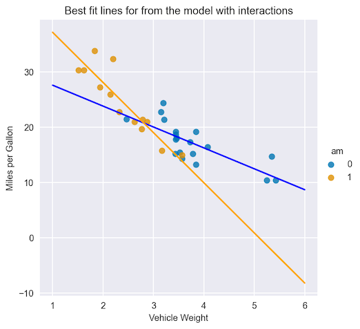
Figure 1 shows a scatterplot that represents the relationship between miles per gallon (target) and the weight of a vehicle (feature). The relationship is quite different depending on the transmission type (another feature).

Line plot showing the best fit lines for vehicle transmission types. They clearly have different slopes.
Figure 1. Best fit lines for vehicle transmission type, including interaction terms

Improving linear model accuracy

Without using interaction terms, a linear model would not be able to capture such a complex relationship. Effectively, it would assign the same coefficient for the weight feature, regardless of the type of transmission. Figure 1 shows the coefficients (slope of the line) by weight feature, which are drastically different for different transmission types.

To overcome this fallacy and make the linear model more flexible, add interaction terms. In general, they are a multiplication of the original features. By adding these new variables to the regression model, you can measure the effects of the interaction between them and the target. 

Interaction terms in time series forecasting

Interaction terms make linear models more flexible. The following example shows how they work in the context of time series forecasting.

Prerequisites

First, load the required libraries:

import numpy as np
import pandas as pd

from sklearn.linear_model import LinearRegression

import seaborn as sns
import matplotlib.pyplot as plt

Dataset generation

Then, generate some artificial time series data with the following characteristics:

  • 10 years of daily data
  • Repeating patterns (seasonality) present in the time series
  • A decreasing trend over the first 7 years
  • No trend in the last 3 years
  • Random noise, added as the last step
# for reproducibility
np.random.seed(42)

# generate the DataFrame with dates
range_of_dates = pd.date_range(
   start="2010-01-01",
   end="2019-12-30"
)
df = pd.DataFrame(index=range_of_dates)

# create a sequence of day numbers
df["linear_trend"] = range(len(df))
df["trend"] = 0.004 * df["linear_trend"].values[::-1]
df.loc["2017-01-01":, "trend"] = 4

# generate the components of the target
signal_1 = 10 + 4 * np.sin(df["linear_trend"] / 365 * 2 * np.pi)
noise = np.random.normal(0, 0.85, len(df))

# combine them to get the target series
df["target"] = signal_1 + noise + df["trend"]

# plot
df["target"].plot(title="Generated time series");

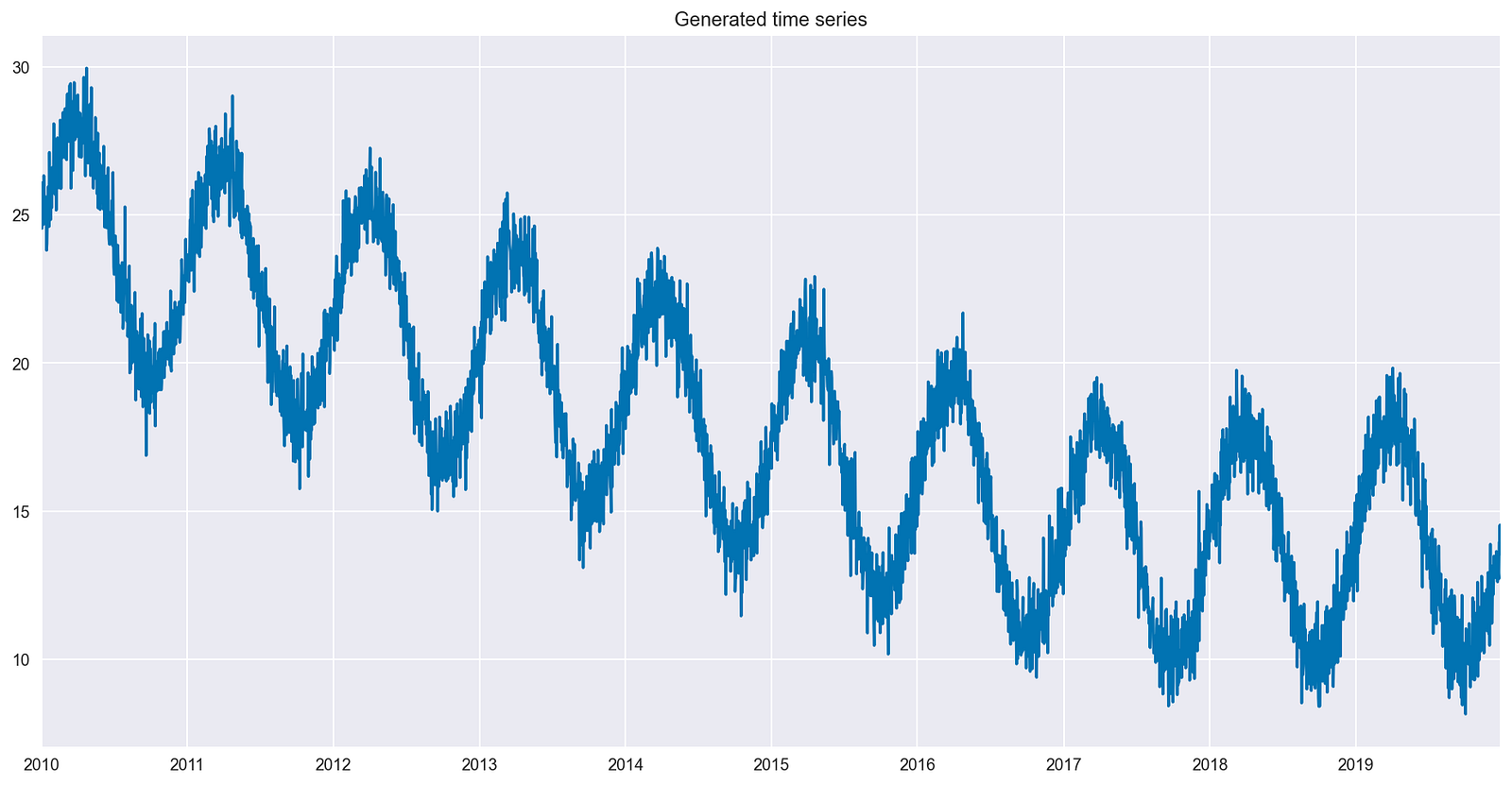
Figure 2 shows the generated time series, which includes all the desired characteristics.

A time series plot including all the desired characteristics, with a slight downward trend over time and containing multiple increases and decreases
Figure 2. The generated time series

Training the benchmark model

Now train a linear model and inspect the best fit line. For this step, create very simple models with a few features. This enables you to visually inspect the impact of the interaction term on the model’s fit.

The simplest model possible contains one feature — an indicator of the passage of time. The linear_trend column created for the time series is effectively the row number of the DataFrame (ordered by date).

X = df[["linear_trend"]]
y = df[["target"]]

lm = LinearRegression()
lm.fit(X, y)

df["model_1"] = lm.predict(X)

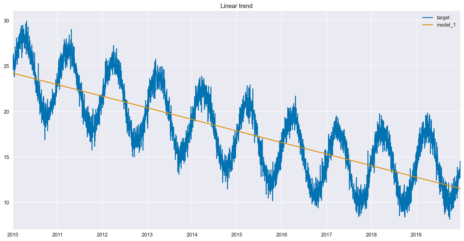
df[["target", "model_1"]].plot(title="Linear trend");

It is worth mentioning that the point is not to properly evaluate the forecasts using separate train and test sets, but rather to explain the impact of the interaction terms on the model’s fit. It is easier to observe the interaction term’s impact by inspecting the fitted values (prediction on the training set) and comparing those fitted values to the original time series. 

Figure 3 shows that the linear model identified a decreasing trend for the entire time series. At the same time, the fit seems off for the last 3 years of data, as there is no trend there.

The plot shows that the fitted line is the same for the entire dataset, thus not capturing the pattern change in the last 3 years.
Figure 3. Best fit line obtained from a linear model using linear trend as a feature

Add a breakpoint

Next, try to make the model learn the new pattern (trend change) using feature engineering. To do so, create a breakpoint, which is a placeholder variable indicating whether a given observation is after January 1, 2017. In this case, the exact point in time when the trend change happened is known. 

Next, train another linear model, this time with two features:

df["after_2017_breakpoint"] = np.where(df.index >= pd.Timestamp('2017-01-01'), 1, 0)

X = df[["linear_trend", "after_2017_breakpoint"]]
y = df[["target"]]

lm = LinearRegression()
lm.fit(X, y)

df["model_2"] = lm.predict(X)

df[["target", "model_2"]].plot(title="Linear trend + breakpoint");
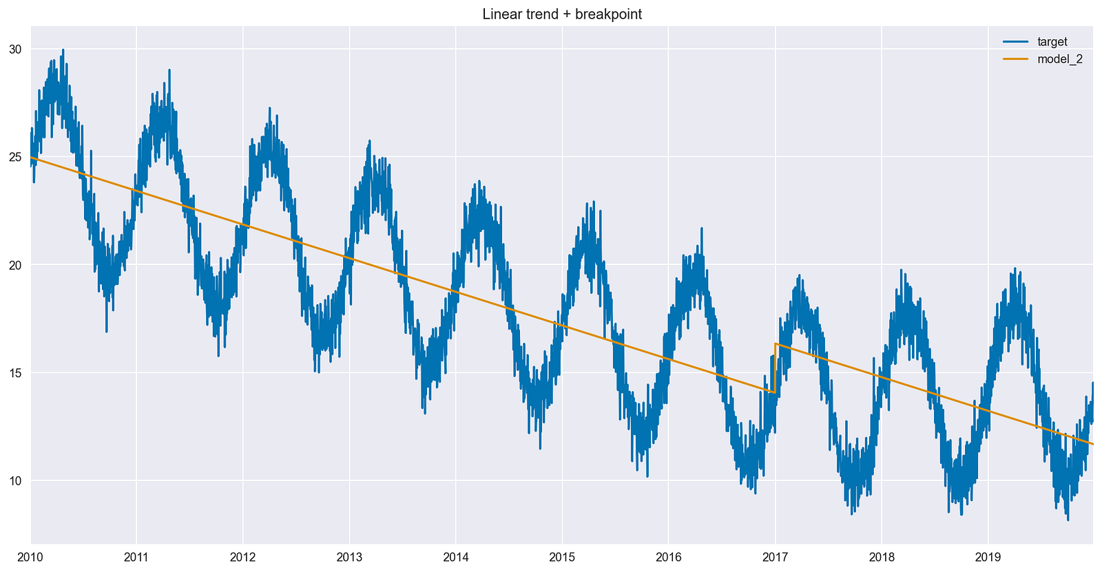
After introducing the breakpoint, there was a vertical jump in the fitted line, but the slope before/after is the same.
Figure 4. Best fit line obtained from a linear model using linear trend and a breakpoint as features

Figure 4 shows a few important changes, as listed below:

  • The fitted line displays a vertical jump, which corresponds to the coefficient by the new Boolean feature.
  • The vertical jump occurs exactly on the first date when the feature becomes active (a value of 1 instead of 0).
  • The slope of the line is the same before and after the introduced breakpoint.
  • The model is trying to compensate for the incorrect slope by adding a fixed amount to the predictions after the breakpoint.

There is no trend in the last 3 years of data, so ideally the line should be close to flat after January 1, 2017. 

Adding an interaction term

To change the slope after the breakpoint, add a more complex dependency on the timestamp (represented by a linear trend). That is exactly what an interaction term does–it is a multiplication of the linear trend and the placeholder variable.

df["interaction_term"] = df["after_2017_breakpoint"] * df["linear_trend"]

X = df[["linear_trend", "after_2017_breakpoint", "interaction_term"]]
y = df[["target"]]

lm = LinearRegression()
lm.fit(X, y)

df["model_3"] = lm.predict(X)

df[["target", "model_3"]].plot(title="Linear trend + breakpoint + interaction term");
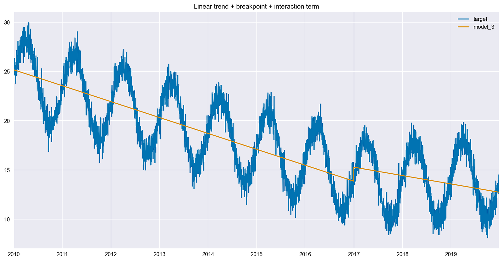
After introducing the interaction term, the slope clearly changes after the breakpoint. It is not as steep anymore.
Figure 5. Best fit line obtained from a linear model using a linear trend, a breakpoint, and an interaction term as features

Figure 5 shows the impact of having the interaction term in the model. Compared to Figure 4, the slope of the best fit line is different after the breakpoint. 

To be more precise, the difference is actually the value of the coefficient by the interaction term. While the new line did not flatten out, it is still less steep than it used to be in the earlier parts of the time series.

Introducing the breakpoint together with an interaction term increased the model’s ability to capture the trend of the time series. In turn, that should increase the predictive performance of the model.

Summary

Using interaction terms can make the specification of a linear model more flexible (different slopes for different lines), which can result in a better fit to the data and better predictive performance. You can add interaction terms as a multiplication of the original features. In the context of time series, you can use interaction terms to better capture any changes to the trend.

Find the code used in this post in A Comprehensive Guide on Interaction Terms in Time Series Forecasting on GitHub. Additionally, the code in the notebook shows how to leverage cuDF and cuML to train your models using GPU acceleration. As always, feedback is welcome. You can reach out to me on Twitter or in the comments.

Categories
Misc

So, So Fresh: Play the Newest Games in the Cloud on Day One

It’s a party this GFN Thursday with several newly launched titles streaming on GeForce NOW. Revel in gaming goodness with Xenonauts 2, Viewfinder and Techtonica, among the four new games joining the cloud this week. Portal fans, stay tuned — the Portal: Prelude RTX mod will be streaming on GeForce NOW to members soon. Plus, Read article >

Categories
Misc

OCI Accelerates HPC, AI, and Database Using RoCE and NVIDIA ConnectX

Oracle is one of the top cloud service providers in the world, supporting over 22,000 customers and reporting revenue of nearly $4 billion per quarter and…
Oracle is one of the top cloud service providers in the world, supporting over 22,000 customers and reporting revenue of nearly $4 billion per quarter and annual growth of greater than 40%. Oracle Cloud Infrastructure (OCI) is growing at an even faster rate and offers a complete cloud infrastructure for every workload. 

Having added 11 regions in the last 18 months, OCI currently offers 41 regions and supports hosted, on-premises, hybrid, and multi-cloud deployments. It enables customers to run a mix of custom-built, third-party ISVs and Oracle applications on a scalable architecture. OCI provides scalable networking and tools to support security, observability, compliance, and cost management. 

One of the differentiators of OCI is its ability to offer high-performance computing (HPC), Oracle Exadata and Autonomous Database, and GPU-powered applications such as AI and machine learning (ML), with fast infrastructure-as-a-service (IaaS) performance that rivals dedicated on-premises infrastructure. A key component to delivering this high performance is a scalable, low-latency network that supports remote direct memory access (RDMA). For more details, see First Principles: Building a High-Performance Network in the Public Cloud.

Networking challenge of HPC and GPU-powered compute 

A commonality across HPC applications, GPU-powered AI workloads, and the Oracle Autonomous Database on Exadata is that they all run as distributed workloads. Data processing occurs simultaneously on multiple nodes, using a few dozen to thousands of CPUs and GPUs. These nodes must communicate with each other, share intermediate results in multi-stage problem solving with gigabytes to petabytes of storage to access common data, and often assemble the results of distributed computing into a cohesive solution. 

These applications require high throughput and low latency to communicate across nodes to solve problems quickly. Amdahl’s law states that the speedup from parallelizing a task is limited by how much of the task is inherently serial and cannot be parallelized. The amount of time needed to transfer information between nodes adds inherently serial time to the task because nodes must wait for the data transfer to complete and for the slowest node in the task to finish before starting the next parallelizable part of the job. 

For this reason, the performance of the cluster network becomes paramount, and an optimized network can enable a distributed compute cluster to deliver results much sooner than the same computing resources running on a slower network. This time-saving speeds job completion and reduces costs. 

What is RDMA? 

RDMA is remote direct memory access, the most efficient means of transferring data between different machines. It enables a server or storage appliance to communicate and share data over a network without making extra copies and without interrupting the host CPU. It is used for AI, big data, and other distributed technical computing workloads. 

Traditional networking interrupts the CPU multiple times and makes multiple copies of the data being transmitted as it passes from the application through the OS kernel, to the adapter, then back up the stack on the receiving end. RDMA uses only one copy of the data on each end and typically bypasses the kernel, placing data directly in the receiving machine’s memory without interrupting the CPU. 

This process enables lower latency and higher throughput on the network and lower CPU utilization for the servers and storage systems. Today, the majority of HPC, technical computing, and AI applications can be accelerated by RDMA. For more details, see How RDMA Became the Fuel for Fast Networks.

What is InfiniBand? 

InfiniBand is a lossless network optimized for HPC, AI, big data, and other distributed technical computing workloads. It typically supports the highest bandwidth available (currently 400 Gbps per connection) for data center networks and RDMA, enabling machines to communicate and share data without interrupting the host CPU. 

InfiniBand adapters offload networking and data movement tasks from the CPU and feature an optimized, efficient networking stack, enabling CPUs, GPUs, and storage to move data rapidly and efficiently. The InfiniBand adapters and switches can also perform specific compute and data aggregation tasks in the network, mostly oriented around message passing interface (MPI) collective operations. 

This in-network computing speeds up distributed applications, enabling faster problem solving. It also frees up server CPU cores and improves energy efficiency. InfiniBand can also automatically balance traffic loads and reroute connections around broken links. 

As a result, many computing clusters that are dedicated to AI, HPC, big data, or other scientific computing run on an InfiniBand network to provide the highest possible performance and efficiency. When distributed computing performance is the top priority, and the adoption of a specialized stack of network adapters, switches, and management is acceptable, InfiniBand is the network of choice. But a data center might choose to run Ethernet instead of InfiniBand, for other reasons.

What is RoCE? 

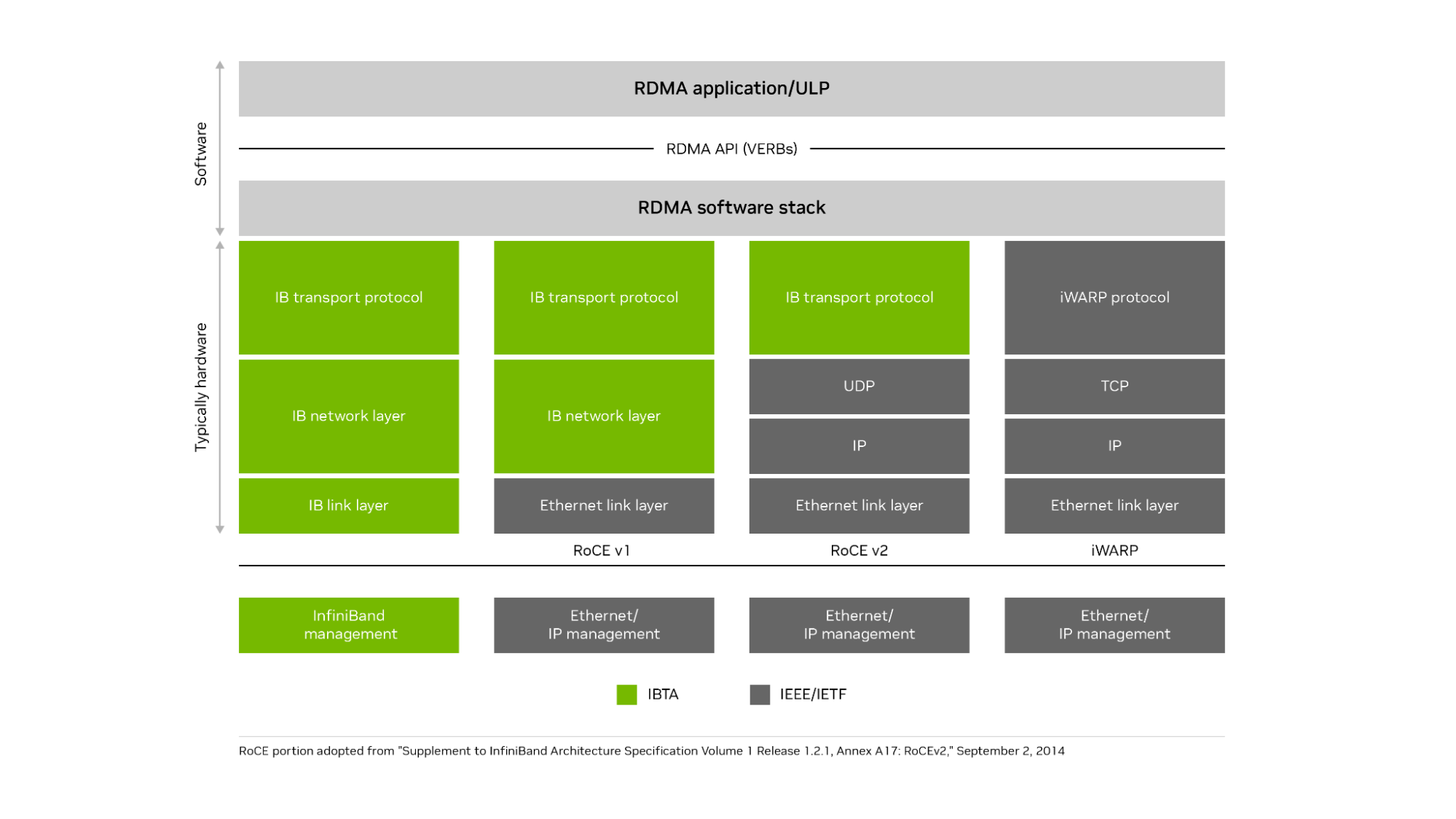
RDMA over Converged Ethernet (RoCE) is an open standard enabling remote direct memory access and network offloads over an Ethernet network. The current and most popular implementation is RoCEv2. It uses an InfiniBand communication layer running on top of UDP (Layer 4) and IP (Layer 3), which runs on top of high-speed Ethernet (Layer 2) connections. 

It also supports remote direct memory access, zero-copy data transfers, and bypassing the CPU when moving data. Using the IP protocol on Ethernet enables RoCEv2 to be routable over standard Ethernet networks. RoCE brings many of the advantages of InfiniBand to Ethernet networks. RoCEv2 runs the InfiniBand transport layer over UDP and IP protocols on an Ethernet network. iWARP ran the iWARP protocol on top of the TCP protocol on an Ethernet network but failed to gain popular adoption because of performance and implementation challenges (Figure 1).

A graphic depicting the OSI transport layer mapped across the RDMA software stack for InfiniBand and Ethernet.
Figure 1. NVIDIA InfiniBand runs the InfiniBand transport layer over an InfiniBand network

How do RoCE networks address scalability?

RoCE operates most efficiently on networks with very low levels of packet loss. Traditionally, small RoCE networks use priority flow control (PFC), based on the IEEE 802.1Qbb specification, to make the network lossless. If any destination is too busy to process all incoming traffic, it sends a pause frame to the next upstream switch port, and that switch holds traffic for the time specified in the pause frame. 

If needed, the switch can also send a pause frame up to the next switch in the fabric and eventually onto the originator of the traffic flow. This flow control avoids having the port buffers overflow on any host or switch and prevents packet loss. You can manage up to eight traffic classes with PFC, each class having its own flows and pauses separate from the others. 

However, PFC has some limitations. It operates only at the Layer 2 (Ethernet) level of the Open System Interconnection (OSI) 7-layer model, so it cannot work across different subnets. While a subnet can have thousands or millions of nodes, a typical subnet is limited to 254 IP addresses and consists of a few racks (often one rack) within a data center, which does not scale for large distributed applications. 

PFC operates on a coarse-grained port level and cannot distinguish between flows sharing that port. Also, if you use PFC in a multi-level switch fabric, congestion at one destination switch for one flow can spread to multiple switches and block unrelated traffic flows that share one port with the congested flow. The solution is usually to implement a form of congestion control.

Congestion management for large RoCE networks

The TCP protocol includes support for congestion management based on dropped packets. When an endpoint or switch is overwhelmed by a traffic flow, it drops some packets. When the sender fails to receive an acknowledgment from the transmitted data, the sender assumes the packet was lost because of network congestion, slows its rate of transmission, and retransmits the presumably lost data. 

This congestion management scheme does not work well for RDMA on Ethernet (and therefore for RoCE). RoCE does not use TCP and  the process of waiting for packets to timeout and then retransmitting the lost data introduces too much latency—and too much variability in latency or jitter—for efficient RoCE operation. 

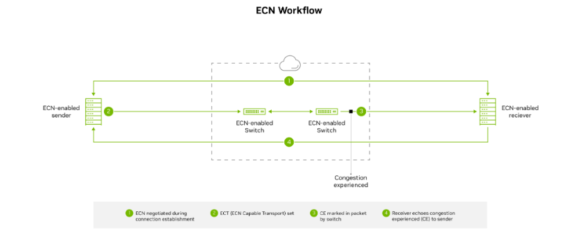
Large RoCE networks often implement a more proactive congestion control mechanism known as explicit congestion notification (ECN), in which the switches mark packets if congestion occurs in the network. The marked packets alert the receiver that congestion is imminent, and the receiver alerts the sender with a congestion notification packet or CNP. After receiving the CNP, the sender knows to back off, slowing down the transmission rate temporarily until the flow path is ready to handle a higher rate of traffic. 

Congestion control works across Layer 3 of the OSI model, so it functions across different subnets and scales up to thousands of nodes. However, it requires setting changes to both switches and adapters supporting RoCE traffic. Implementation details of when switches mark packets for congestion, how quickly senders back off sending data, and how aggressively senders resume high-speed transmissions are all critical to determining the scalability and performance of the RoCE network.

A graphic depicting ECN workflow mapping the progress of experiencing congestion, marketing the packet within the switch, and notifying the sender.
Figure 2. ECN marks outgoing packets as CE–Congestion Experienced when the switch queue is becoming full. The flow recipient receives the packet and notifies the sender to slow transmission

Other Ethernet-based congestion control algorithms include quantized congestion notification (QCN) and data center TCP (DCTCP). In QCN, switches notify flow senders directly with the level of potential congestion, but the mechanism functions only over L2. Consequently, it cannot work across more than one subnet. DCTCP uses the sender’s network interface card (NIC) to measure the round-trip time (RTT) of special packets to estimate how much congestion exists and how much the sender must slow down data transmissions. 

But DCTCP lacks a fast start option to quickly start or resume sending data when no congestion exists, places a heavy load on host CPUs, and does not have a good mechanism for the receiver to communicate with the sender. In any case, DCTCP requires TCP, so it does not work with RoCE. 

Smaller RoCE networks using newer RDMA-capable ConnectX SmartNICs from NVIDIA, or newer NVIDIA BlueField DPUs, can use Zero Touch RoCE (ZTR). ZTR enables excellent RoCE performance without setting up PFC or ECN on the switch, which greatly simplifies network setup. However, initial deployments of ZTR have been limited to small RoCE network clusters, and a more scalable version of ZTR that uses RTT for congestion notification is still in the proving stages. 

How OCI implements a scalable RoCE network 

OCI determined that certain cloud workloads required RDMA for maximum performance. These include AI, HPC, Exadata, autonomous databases, and other GPU-powered applications. Out of the two standardized RDMA options on Ethernet, they chose RoCE for its performance and wider adoption. 

The RoCE implementation needed to scale to run across clusters containing thousands of nodes and deliver consistently low latency to ensure an excellent experience for cloud customers. 

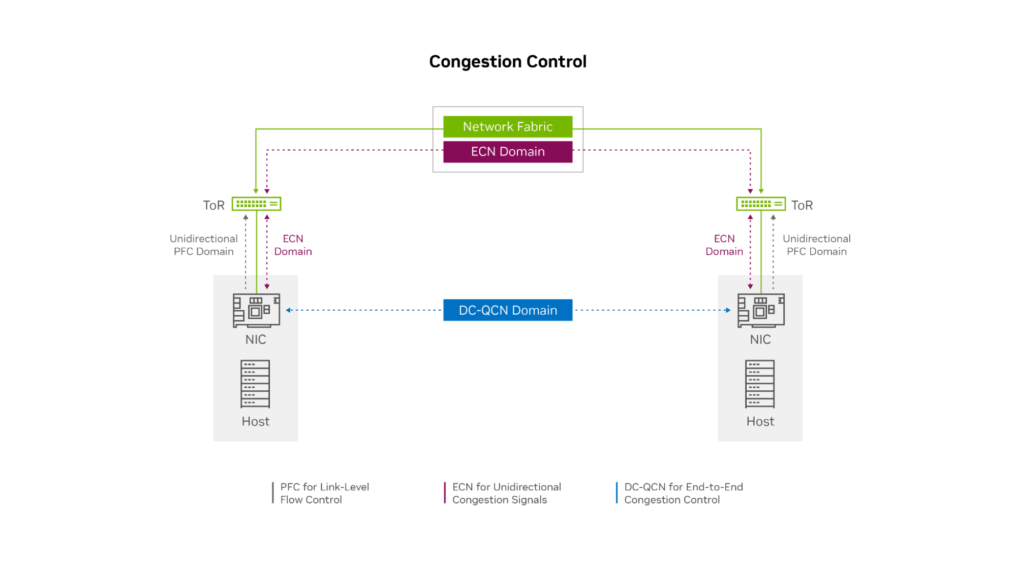
After substantial research, testing, and careful design, OCI decided to customize their own congestion control solution based on the data center quantized congestion notification (DC-QCN) algorithm, which they optimized for different RoCE-accelerated application workloads. The OCI DC-QCN solution is based on ECN with minimal use of PFC.

A graph shows how the OCI network uses RoCE with priority flow control at the link level, explicit congestion notification for unidirectional congestion signaling and data center quantized congestion notification for end-to-end congestion control.
Figure 3. The OCI RoCE network uses ECN across the network fabric plus a limited amount of unidirectional PFC only between the hosts and ToR switches

A separate network for RoCE 

OCI built a separate network for RoCE traffic because the needs of the RDMA network tend to differ from the regular data center network. The different types of application traffic, congestion control, and routing protocols each prefer to have their own queues. Each NIC typically supports only eight traffic classes, and the NIC and switch configuration settings and firmware might be different for RDMA from non-RDMA workloads. For these reasons, having a separate Ethernet network for RoCE traffic and RoCE-accelerated applications makes sense. 

Limited use of PFC at the edge

OCI implemented a limited level of PFC, only unidirectionally at the network edge. Endpoints can ask the top-of-rack (ToR) switch to pause transmission if their NICs buffer fills up. However, the ToR switches never ask the endpoints to pause and do not pass ‌pause requests up the network to leaf or spine switches. This process prevents head-of-line blocking and congestion spreading if the incoming traffic flow rate temporarily exceeds the receiver’s ability to process and buffer data. 

The ECN mechanism ensures that PFC is very rarely needed. In the rare case that a receiving node’s NIC buffer is temporarily overrun while the ECN feedback mechanism is activating, PFC enables the receiving node to briefly pause the incoming data flow until the sender receives the CNPs and slows its transmission rate. 

In this sense, you can use PFC as a last resort safeguard to prevent buffer overrun and packet loss at the network edge (at the endpoints). OCI envisions that with the next generation of ConnectX SmartNICs, you might not need PFC, even at the edge of the network. 

Multiple classes of congestion control 

OCI determined that they need at least three customized congestion control profiles within DC-QCN for different workloads. Even within the world of distributed applications that require RDMA networking, the needs vary across the following categories:

  • Latency sensitive, requiring consistently low latency throughput
  • Sensitive, high throughput
  • Mixed, requires a balance of low-latency and high throughput

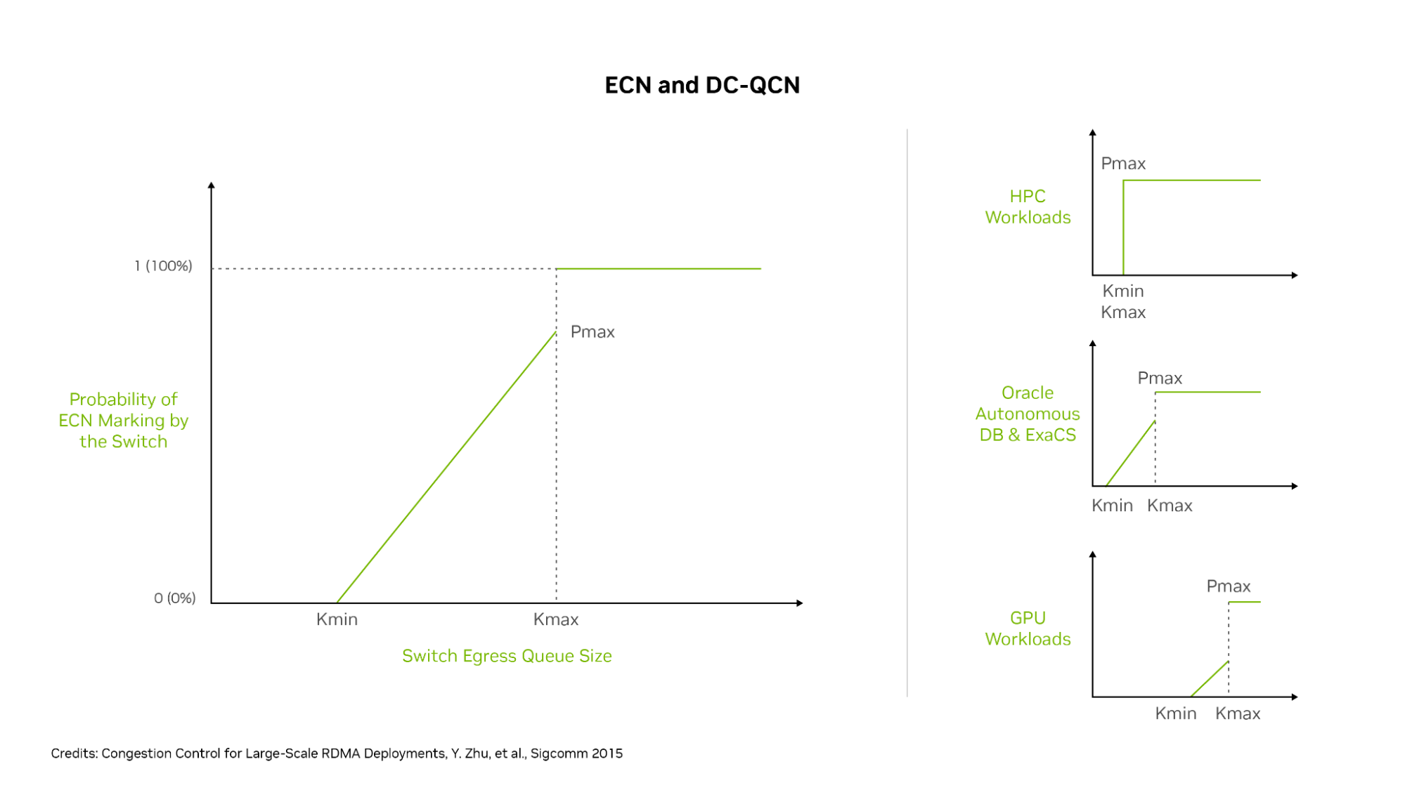
The primary setting for customizing congestion control is the probability P (ranging from 0 to 1) of the switch adding the ECN marking to an outgoing packet, based on queue thresholds Kmin and Kmax. P starts at 0 when the switch queue is not busy, which means it has no chance of congestion. 

When the port queue reaches Kmin, the value P rises above 0, increasing the chance that any packet is marked with ECN. When the queue fills to value Kmax, P is set to Pmax (typically 1), meaning every outgoing packet of that flow on that switch is marked with ECN. Different DC-QCN profiles typically have a no-congestion range where P is 0, a potential congestion range where P is between 0 and 1, and a congestion range where P is 1. 

A more aggressive set of thresholds has lower values for Pmin and Pmax, resulting in earlier ECN packet marking and lower latency but possibly also lower maximum throughput. A relaxed set of thresholds has higher values for Pmin and Pmax, marking fewer packets with ECN, resulting in some higher latencies but also higher throughput. 

To the right side of Figure 4 are three examples of OCI workloads: HPC, Oracle Autonomous DataBase and Exadata Cloud Service, and GPU workloads. These services use different RoCE congestion control profiles. HPC workloads are latency-sensitive and give up some throughput to guarantee lower latency. ‌Consequently, Kmin and Kmax are identical and low (aggressive), and at a low amount of queuing, they mark 100% of all packets with ECN. 

Most GPU workloads are more forgiving on latency but need maximum throughput. The DC-QCN profile gradually marks more packets as buffers ramp from Kmin to Kmax and sets those values relatively higher to enable switch buffers to get closer to full before signaling to flow endpoints that they slow down. 

For Autonomous Database and Exadata Cloud Service workloads, the required balance of latency and bandwidth is in between. Marking or increasing P value gradually increases between Kmin and Kmax, but these values are set at lower threshold values than for GPU workloads.  

A graphic showing four line graphs comparing how optimal network congestion control is achieved by varying data center quantized congestion notification thresholds on different services.
Figure 4. OCI sets DC-QCN to use different Kmin and Kmax thresholds for ECN packet marking, resulting in optimized network behavior on their RoCE network for different workloads

With these settings, HPC flows get 100% ECN packet marking as soon as the queues hit the Kmin level (which is the same here as Kmax) for early and aggressive congestion control engagement. Oracle Autonomous Database and Exadata flows see moderately early ECN marking, but only a portion of packets is marked until buffers reach the Kmax level. 

Other GPU workloads have a higher Kmin setting so ECN marking does not begin until switch queues are relatively fuller, and 100% ECN marking only happens when the queues are close to full. Different workloads get the customized congestion control settings needed to provide the ideal balance of latency and throughput for maximum application performance. 

Leveraging advanced network hardware

An important factor in achieving high performance for RoCE networks is the type of network card used. The NIC offloads the networking stack, including RDMA, to a specialized chip to offload the work from the CPUs and GPUs. OCI uses ConnectX SmartNICs, which have market-leading network performance for both TCP and RoCE traffic. 

These SmartNICs also support rapid PFC and ECN reaction times for detecting ECN-marked packets or PFC pause frames, sending CNPs, and adjusting the data transmission rates downward and upward in response to congestion notifications. 

NVIDIA has been a long time leader in the development and support of RDMA, PFC, ECN, and DC-QCN technology, and a leader in high-performance GPUs and GPU connectivity. The advanced RoCE offloads in ConnectX enable higher throughput and lower latency on the OCI network, and their rapid, hardware-based ECN reaction times help ensure that DC-QCN functions smoothly.

By implementing an optimized congestion control scheme on a dedicated RoCE network, plus a combination of localized PFC, multiple congestion control profiles, and NVIDIA network adapters, OCI has built a very scalable cluster network. It’s ideal for distributed workloads, such as AI and ML, HPC, and Oracle Autonomous Database, and delivers high throughput and low-latency performance close to what an InfiniBand network can achieve.  

Emphasizing data locality

With optimizing cluster network performance, OCI also manages data locality to minimize latency. With the large size of RoCE-connected clusters that often span multiple data center racks and halls, even in an era of 100-, 200-, and 400-Gbps networking connections, the speed of light has not changed, and longer cables result in higher latency. 

Connections to different halls in the data center traverse more switches, and each switch hop adds some nanoseconds to connection latency. OCI shares server locality information with both its customers and the job scheduler, so they can schedule jobs to use servers and GPUs that are close to each other in the network. 

For example, the NVIDIA Collective Communication Library (NCCL) understands the OCI network topology and server locality information and can schedule GPU work accordingly. So, the compute and storage connections traverse fewer switch hops and shorter cable lengths, to reduce the average latency within the cluster. 

It also sends less traffic to spine switches, simplifying traffic routing and load-balancing decisions. OCI also worked with its switch vendors to make the switches more load-aware, so flows can be routed to less-busy connections. Each switch generally has two connections up and down the network, enabling multiple datapaths for any flow. 

Conclusion

By investing in a dedicated RoCE network with an optimized implementation of DC-QCN, advanced ConnectX NICs, and customized congestion control profiles, OCI delivers a highly scalable cluster that supports accelerated computing for many different workloads and applications. OCI cluster networks simultaneously deliver high throughput and low latency. For small clusters, latency-half the round trip time-can be as little as 2 microseconds. For large clusters, latency is typically under 4 microseconds. For extremely large superclusters, latencies are in the range of 4-8 microseconds, with most traffic seeing latencies at the lower end of this range. 

Oracle Cluster Infrastructure uses an innovative approach to deliver scalable, RDMA-powered networking on Ethernet for a multitude of distributed workloads, providing higher performance and value to their customers. 

For more information, see the following resources:

Categories
Misc

Programming the Quantum-Classical Supercomputer

Heterogeneous computing architectures—those that incorporate a variety of processor types working in tandem—have proven extremely valuable in the continued…
Heterogeneous computing architectures—those that incorporate a variety of processor types working in tandem—have proven extremely valuable in the continued scalability of computational workloads in AI, machine learning (ML), quantum physics, and general data science. 

Critical to this development has been the ability to abstract away the heterogeneous architecture and promote a framework that makes designing and implementing such applications more efficient. The most well-known programming model that accomplishes this is CUDA Toolkit, which enables offloading work to thousands of GPU cores in parallel following a single-instruction, multiple-data model. 

Recently, a new form of node-level coprocessor technology has been attracting the attention of the computational science community: the quantum computer, which relies on the non-intuitive laws of quantum physics to process information using principles such as superposition, entanglement, and interference. This unique accelerator technology may prove useful in very specific applications and is poised to work in tandem with CPUs and GPUs, ushering in an era of computational advances previously deemed unfeasible. 

The question then becomes: If you enhance an existing classically heterogeneous compute architecture with quantum coprocessors, how would you program it in a manner fit for computational scalability?

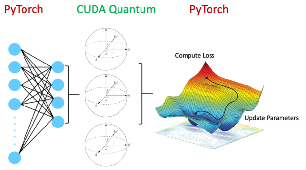
NVIDIA is answering this question with CUDA Quantum, an open-source programming model extending both C++ and Python with quantum kernels intended for compilation and execution on quantum hardware. 

This post introduces CUDA Quantum, highlights its unique features, and demonstrates how researchers can leverage it to gather momentum in day-to-day quantum algorithmic research and development. 

CUDA Quantum: Hello quantum world 

To begin with a look at the CUDA Quantum programming model, create a two-qubit GHZ state with the Pythonic interface. This will accustom you to its syntax.

import cudaq

# Create the CUDA Quantum Kernel
kernel = cudaq.make_kernel()

# Allocate 2 qubits
qubits = kernel.qalloc(2)

# Prepare the bell state
kernel.h(qubits[0]) 
kernel.cx(qubits[0], qubits[1])

# Sample the final state generated by the kernel 
result = cudaq.sample(kernel, shots_count = 1000) 

print(result) 

{11:487, 00:513}

The language specification borrows concepts that CUDA has proven successful; specifically, the separation of host and device code at the function boundary level. The code snippet below demonstrates this functionality on a GHZ state preparation example in C++. 

#include 

int main() {
      // Define the CUDA Quantum kernel as a C++ lambda
	auto ghz =[](int numQubits) __qpu__ {
           // Allocate a vector of qubits
		cudaq::qvector q(numQubits);

           // Prepare the GHZ state, leverage standard 
           // control flow, specify the x operation 
           // is controlled. 
		h(q[0]);
		for (int i = 0; i (q[i], q[i + 1]);
	};

     // Sample the final state generated by the kernel
auto results = cudaq::sample(ghz, 15); 
results.dump();

return 0;
}

CUDA Quantum enables the definition of quantum code as stand-alone kernel expressions. These expressions can be any callable in C++ (a lambda is shown here, and implicitly typed callable) but must be annotated with the __qpu__ attribute enabling the nvq++ compiler to compile them separately. Kernel expressions can take classical input by value (here the number of qubits) and leverage standard C++ control flow, for example for loops and if statements. 

The utility of GPUs

The experimental efforts to scale up QPUs and move them out of research labs and host them on the cloud for general access have been phenomenal. However, current QPUs are noisy and small-scale, hindering advancement of algorithmic research. To aid this, circuit simulation techniques are answering the pressing requirements to advance research frontiers. 

Desktop CPUs can simulate small-scale qubit statistics; however, memory requirements of the state vector grow exponentially with the number of qubits. A typical desktop computer possesses eight GB of RAM, enabling one to sluggishly simulate approximately 15 qubits. The  latest NVIDIA DGX H100 enables you to surpass the 35-qubit mark with unparalleled speed. 

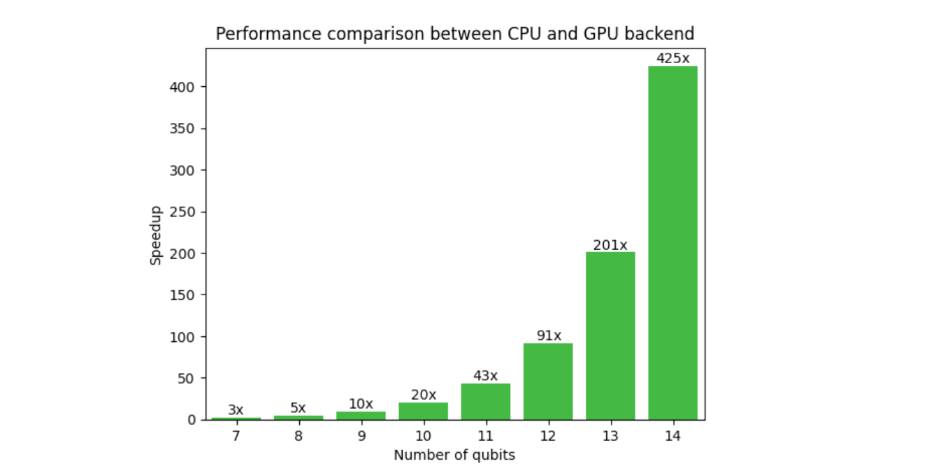
Figure 1 shows a comparison of CUDA Quantum on CPU and GPU backend for a typical variational algorithmic workflow. The need for GPUs is evident here, as the speedup at 14 qubits is 425x and increases with qubit count. Extrapolating to 30 qubits, the CPU-to-GPU runtime is 13 years, compared to 2 days. This unlocks researchers’ abilities to go beyond small-scale proof of concept results to implementing algorithms closer to real-world applications.

Bar graph showing performance improvements in execution time between a CPU and GPU as a function of number of qubits. At 14 qubits, the GPU is 425 times faster than the CPU.
Figure 1. Performance comparison between CPU and GPU for a typical quantum neural network workflow as a function of qubit count 

Along with CUDA Quantum, NVIDA has developed cuQuantum, a library enabling lightning-fast simulation of a quantum computer using both state vector and tensor network methods through hand-optimized CUDA kernels. Memory allocation and processing happens entirely on GPUs resulting in dramatic increases in performance and scale. CUDA Quantum in combination with cuQuantum forms a powerful platform for hybrid algorithm research. 

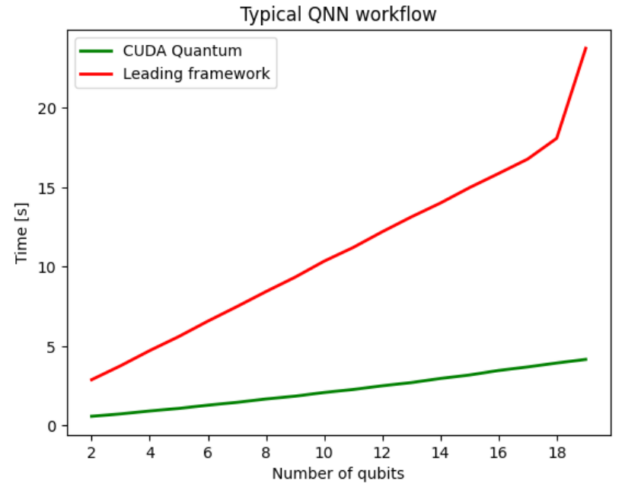
Figure 2 compares CUDA Quantum with a leading quantum computing SDK, both leveraging the NVIDIA cuQuantum backend to optimally offload circuit simulation onto NVIDIA GPUs. In this case, the benefits of using CUDA Quantum are isolated and yield a 5x performance improvement on average compared to a leading framework. 

 Line plot showing the execution time for a typical quantum neural network workflow as a function of number of qubits for CUDA Quantum and a leading framework. CUDA Quantum is on average 5x faster. Since both frameworks were executed on GPUs, we are isolating the performance benefits of using CUDA Quantum.
Figure 2. GPU-to-GPU comparison between CUDA Quantum and a leading framework, both offloading circuit simulation to NVIDIA GPUs, with CUDA Quantum on average 5x faster

Enabling multi-QPU workflows of the future

CUDA Quantum is not limited to consideration of current cloud-based quantum execution models, but is fully anticipating tightly coupled, system-level quantum acceleration. Moreover, CUDA Quantum enables application developers to envision workflows for multi-QPU architectures with multi-GPU backends. 

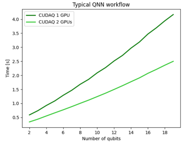
For the preceding quantum neural network (QNN) example, you can use the multi-GPU functionality to run a forward pass of the dataset enabling us to perform multi-QPU workflows of the future. Figure 3 shows results for distributing the QNN workflow across two GPUs and demonstrates strong scaling performance indicating effective usage of all GPU compute resources. Using two GPUs makes the overall workflow twice as fast compared to a single GPU, demonstrating strong scaling. 

Line plot showing the execution time of a typical quantum neural network workflow as a function of the number of qubits. The execution time is approximately half when two GPUs are used in comparison to a single GPU.
Figure 3. ‌Results for distributing the QNN forward pass workload to multiple QPUs enabled ‌by the multi-GPU backend

Another common workflow that benefits from multi-QPU parallelization is the Variational Quantum Eigensolver (VQE). This requires the expectation value of a composite Hamiltonian made up of multiple single Pauli tensor product terms. The CUDA Quantum observe call, shown below, automatically batches terms (Figure 4), and offloads to multiple GPUs or QPUs if available, demonstrating strong scaling (Figure 5). 

numQubits, numTerms = 30, 1e5
hamiltonian = cudaq.SpinOperator.random(numQubits, numTerms)
cudaq.observe(ansatz, hamiltonian, parameters)
Image showing a Hamiltonian composed of many terms being batched into four groups and offloaded to four GPUs.
Figure 4. Automatic batching of Hamiltonian terms across multiple NVIDIA A100 GPUs
Bar graph showing speedup in execution time gained by automatically batching a Hamiltonian composed of multiple terms into four batches and executing on four GPUs. The speedups gained demonstrate strong scaling.
Figure 5. Speedups gained due to an optimized software stack supporting the hardware available to the user, GPUs or QPUs

GPU-QPU workflows 

This post has so far explored using GPUs for scaling quantum circuit simulation beyond what is possible on CPUs, as well as multi-QPU workflows. The following sections dive into true heterogeneous computing with a hybrid quantum neural network example using PyTorch and CUDA Quantum.

As shown in Figure 6, a hybrid quantum neural network encompasses a quantum circuit as a layer within the overall neural network architecture. An active area of research, this is poised to be advantageous in certain areas, improving generalization errors.

Image showing layers of neural network nodes, the output of which acts as the input to a quantum circuit, which is measured to generate the loss function. This workflow enables one to integrate PyTorch layers with CUDA Quantum.
Figure 6. Hybrid quantum neural network architecture accelerated by GPUs made possible by CUDA Quantum

Evidently, it is advantageous to run the classical neural network layers on GPUs and the quantum circuits on QPUs. Accelerating the whole workflow with CUDA Quantum is made possible by setting the following: 

quantum_device = cudaq.set_target('ion-trap')
classical_device = torch.cuda.set_device(gpu0)

The utility of this is profound. CUDA Quantum enables offloading relevant kernels suited for QPUs and GPUs in a tightly integrated, seamless fashion. In addition to hybrid applications, workflows involving error correction, real-time optimal control, and error mitigation through Clifford data regression would all benefit from tightly coupled compute architectures. 

QPU hardware providers 

The foundational information unit embedded within the CUDA Quantum programming paradigm is the qudit, which represents a quantum bit capable of accessing d-states. Qubit is a specific instance where d=2. By using qudits, CUDA Quantum can efficiently target diverse quantum computing architectures, including superconducting circuits, ion traps, neutral atoms, diamond-based, photonic systems, and more. 

You can conveniently develop workflows, and the nvq++ compiler automatically compiles and executes the program on the designated architecture. Figure 7 shows the compilation speedups that the novel compiler yields. Compilation involves circuit optimization, decomposing into the native gate sets supported by the hardware and qubit routing. The nvq++ compiler used by CUDA Quantum is on average 2.4x faster compared to its competition.

Line graph showing how the compilation time scales with number of qubits for CUDA Quantum and a leading framework. The novel ‌compiler used by CUDA Quantum is on average 2.4x faster and its rate of increase (gradient) is also much shallower in comparison.
Figure 7. Compilation time scaling with the number of qubits for CUDA Quantum and a leading framework

To accommodate the desired backend, you can simply modify the set_target() flag. Figure 8 shows an example of how you can seamlessly switch between the simulated backend and the Quantinuum H1 ion trap system. The top shows the syntax to set the desired backend in Python and the bottom in C++. 

Image showing a heatmap of the cost landscape generated by a VQE workflow being executed on cuQuantum simulated backed and the Quantinuum H1 processor. The ease with which users can change the backend and the syntax enabling this in Python and C++ is highlighted.
Figure 8. VQE landscape plots demonstrating execution on simulated or QPU hardware

Getting started with CUDA Quantum

This post has just briefly touched on some of the features of the CUDA Quantum programming model. Reach out to the CUDA Quantum community on GitHub and get started with some example code snippets. We are excited to see the research CUDA Quantum enables for you.