NVIDIA Modulus is a framework for building, training, and fine-tuning deep learning models for physical systems, otherwise known as physics-informed machine…
NVIDIA Modulus is a framework for building, training, and fine-tuning deep learning models for physical systems, otherwise known as physics-informed machine learning (physics-ML) models. Modulus is available as OSS (Apache 2.0 license) to support the growing physics-ML community.
The latest Modulus software update, version 23.05, brings together new capabilities, empowering the research community and industries to develop research into enterprise-grade solutions through open-source collaboration.
Two major components of this update are 1) supporting new network architectures that include graph neural networks (GNNs) and recurrent neural networks (RNNs), and 2) improving the ease of use for AI practitioners.
Graph neural network support
GNNs are transforming how researchers are addressing challenges involving intricate graph structures, such as those encountered in physics, biology, and social networks. By leveraging the structure of graphs, GNNs are capable of learning and making predictions based on the relationships among nodes in a graph.
Through the application of GNNs, researchers can model systems to be represented as graphs or meshes. This capability is useful in applications such as computational fluid dynamics, molecular dynamics simulations, and material science.
Using GNNs, researchers can better understand the behavior of complex systems with complex geometries, and generate more accurate predictions based on the learned patterns and interactions within the data.
The latest version of NVIDIA Modulus includes support for GNNs. This enables you to develop your own GNN-based models for specific use cases. Modulus includes recipes that use the MeshGraphNet architecture based on the work presented in Learning Mesh-Based Simulation with Graph Networks. Such architectures can now be trained in Modulus, which includes a MeshGraphNet model pretrained on a parameterized vortex shedding dataset. This pretrained model is available through NVIDIA NGC.
Modulus also includes the GraphCast architecture proposed in GraphCast: Learning Skillful Medium-Range Global Weather Forecasting. GraphCast is a novel GNN-based architecture for global weather forecasting. It significantly improves on some existing models by effectively capturing spatio-temporal relationships in weather data. The weather data is modeled as a graph, where nodes represent Earth grid cells. This graph-based representation enables the model to capture both local and non-local dependencies in the data.
The architecture of GraphCast consists of four main components: embedder, encoder, processor, and decoder. The embedder component embeds the input features into a latent representation. The encoder maps the local regions of the grid’s latent features into nodes of a multi-mesh graph representation. The processor updates each multi-mesh node using learned message-passing.
Finally, the decoder maps the processed multi-mesh features back onto the grid representation. The multi-mesh is a set of icosahedral meshes with increasing resolution, providing uniform resolution across the globe. A recipe for training GraphCast on the ERA-5 dataset with support for data parallelism is provided in Modulus-Launch. Figure 1 shows the out-of-sample prediction for the 2-meter temperature using a GraphCast model trained in Modulus on a 34-variable subset of the ERA-5 dataset.
Figure 1. The out-of-sample prediction for the 2-meter temperature using a GraphCast model trained in Modulus on a 34-variable subset of the ERA-5 dataset
The GraphCast implementation supports gradient checkpointing for reducing the memory overhead. It also provides several optimizations including CuGraphOps support, fused layer norm and Adam optimizer using Apex, efficient edge feature updates, and more.
Recurrent neural network support
Time-series prediction is a key task in many domains. The application of deep learning architectures—particularly RNNs, long short-term memory networks (LSTMs), and similar networks—has significantly enhanced the predictive capabilities.
These models are unique in their ability to capture temporal dependencies and learn complex patterns over time, making them well suited for forecasting time varying relationships. In physics-ML, these models are critical in predicting dynamic physical systems’ evolution, enabling better simulations, understanding of complex natural phenomena, and aiding in discoveries.
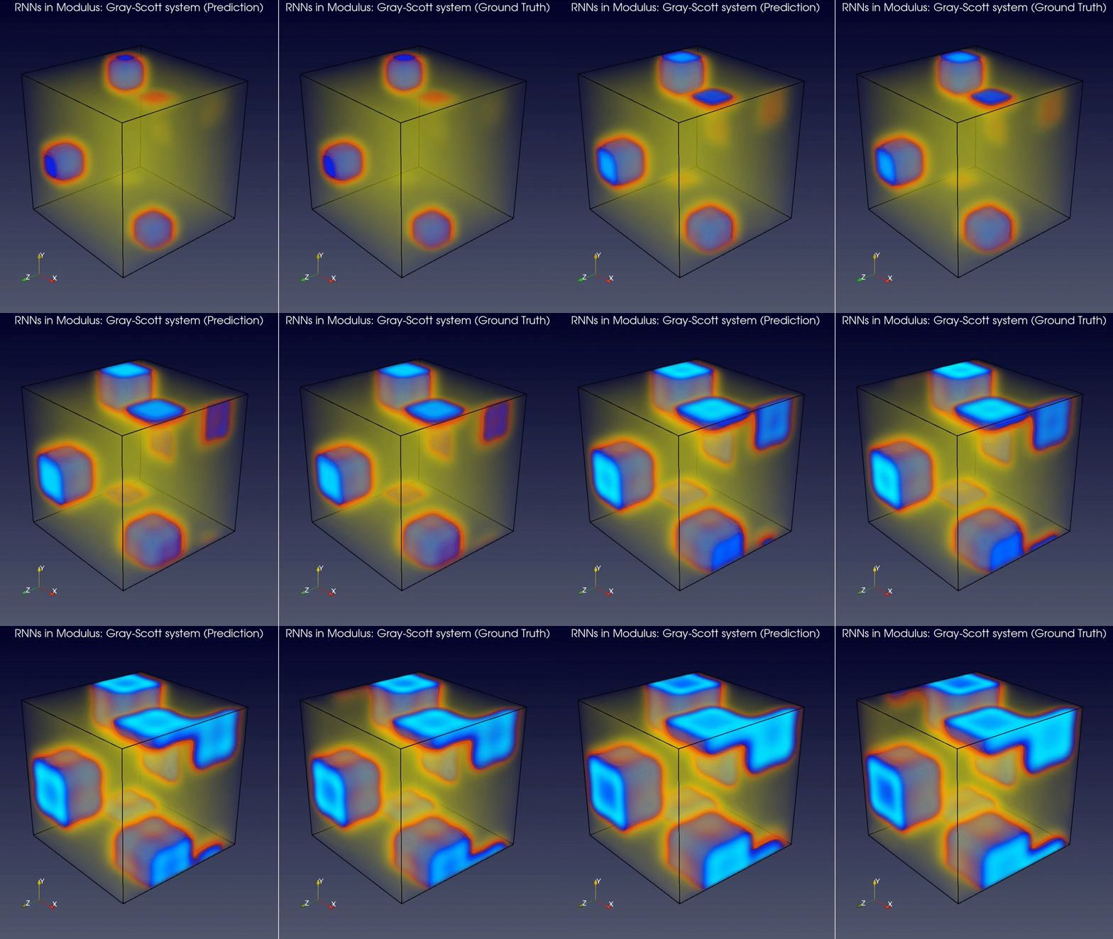
The latest version of Modulus has added support for RNN type layers and models. This enables you to use RNNs for 2D spatial domains and 3D spatial domains in model prediction workflows. Figure 2 shows a comparison between the predictions of a RNN model in Modulus and the ground truth for a Gray-Scott system.
Figure 2. 3D transient predictions on a Gray-Scott system in NVIDIA Modulus
Modules for ease of use
The Modulus codebase has been re-architected into modules to facilitate ease of use. This is in line with PyTorch, which has become one of the most popular deep learning frameworks for researchers over the past few years, given the ease of use.
The core Modulus module consists of the core framework and algorithms for physics-ML models. The Modulus-Launch module consists of optimized training recipes for accelerating PyTorch-like workflows for training models. This module enables AI researchers to have a PyTorch-like experience. NVIDIA Modulus Sym is a module based on the symbolic partial differential equation (PDE) that domain experts can use to train PDE-based physics-ML models.
One key feature of modern deep learning frameworks is their interoperability. This Modulus release makes it easier for AI developers to bring PyTorch models into Modulus and vice versa. This helps to ensure that models can be shared and reused across different platforms and environments.
For more details about all the new features in Modulus 23.05, see the Modulus release notes.
Start using GNNs for physics-ML today
To learn more and get started with NVIDIA Modulus, see the NVIDIA Deep Learning Institute course, Introduction to Physics-Informed Machine Learning with Modulus. Kick-start your Modulus experience with the LaunchPad for Modulus free hands-on lab. With short-term access provided, there is no need to set up your own compute environment.
Voice-enabled technology is becoming ubiquitous. But many are being left behind by an anglocentric and demographically biased algorithmic world. Mozilla Common…
Voice-enabled technology is becoming ubiquitous. But many are being left behind by an anglocentric and demographically biased algorithmic world. Mozilla Common Voice (MCV) and NVIDIA are collaborating to change that by partnering on a public crowdsourced multilingual speech corpus—now the largest of its kind in the world—and open-source pretrained models. It is now easier than ever before to develop automatic speech recognition (ASR) technology that works for speakers of many languages.
Do multilingual NVIDIA NeMo open-source models exist?
Caroline de Brito Gottlieb: To make Speech AI more accessible and serve a global community, we first need to understand how the world uses language. Monolingualism is an anomaly worldwide, so researchers at NVIDIA are focused on creating state-of-the-art AI for multilingual contexts.
Through NeMo, NVIDIA has released its first model for multilingual and code-switched/code-mixed speech recognition, which can transcribe audio samples into English, Latin/North American Spanish, as well as both English and Spanish used in the same sentence—a phenomenon called code-switching, or code-mixing. NVIDIA will soon have a multilingual model on NeMo for Indic languages as well.
The switching or mixing of codes is very common in multilingual communities and communities speaking multiple dialects or varieties of the same language. This poses unique challenges for existing speech AI solutions. However, the open-source NeMo model is an important step toward AI that accurately reflects and supports how global communities actually use speech in real-world contexts.
Do datasets extend beyond “language” to include domain-specific vocabulary? For example, finance and healthcare datasets may differ.
EM Lewis-Jong: Domains represented within the corpora on MCV have been historically driven by communities who choose to create datasets through the platform. That means different languages have varied domains represented in their datasets—some might be heavy on news and media, whereas others might contain more educational text. If you want to enhance domain-specific coverage in a Common Voice dataset, simply go through the process of adding text into the platform through GitHub or the Sentence Collector tool. All domains are welcome.
MCV is actively rebuilding and expanding the Sentence Collector tool to make it easier to ingest large volumes of text, and tag them appropriately. Expect to see these changes in April 2023. Also, the team has been collaborating closely with NVIDIA and other data partners to ensure the metadata schema is as interoperable as possible. Domain tagging the Common Voice corpora is a big part of that.
Caroline de Brito Gottlieb: Accounting for domain-specific language is a critical challenge, in particular when applying AI solutions across industries. That is why NVIDIA Riva offers multiple techniques, such as word boosting and vocabulary extension, for customizing ASR models to improve the recognition of specific words.
Our team primarily thinks of domain as a matter of vocabulary and terminology. This alone is a big challenge, given the different levels of specialized terminology and acronyms like GPU, FTP, and more. But it is also important to collect domain-specific data beyond just individual words to capture grammatical or structural differences; for example, the way negation is expressed in clinical practice guidelines. Designing and curating domain-specific datasets is an active area of collaboration between Common Voice and NVIDIA, and we’re excited to see progress in domain-specific ASR for languages beyond English.
How do you differentiate varied versions of Spanish, English, Portuguese, and other languages across geographies?
EM Lewis-Jong: Historically, MCV didn’t have a great system for differentiating between varied versions of a language. Communities chose between creating an entirely new dataset (organized by language), or they could use the accent field. In 2021, MCV did an intensive research exercise and discovered the following:
Limited community awareness about variants: New communities without much context weren’t always sure about how to categorize themselves. Once they’d made the decision about whether to become a new language dataset or remain as an accent, it was difficult to change their minds.
Dataset fragmentation: Diverse communities, such as those with large diaspora populations, may feel they need to split up entirely and set up a whole new language. This fragments the dataset and confuses contributors.
Identity and experience: Some language communities and contributors make use of accent tags, but can feel marginalized and undermined by this. Talking about language is talking about power, and some people want to have the ability to identify their speech beyond ‘accent’ in ways that respect and represent them.
Linguistic and orthographic diversity: Some communities felt there was no suitable arrangement for them, as their spoken language had multiple writing systems. Currently, MCV assumes a 1:1 relationship between spoken word and written word.
For these reasons, the team enabled a new category on the platform called Variant. This is intended to help communities systematically differentiate within languages, and especially to support large languages with a diverse range of speakers.
Where possible, MCV uses BCP-47 codes for tagging. BCP 47 is a flexible system that enables communities to pull out key information such as region, dialect, and orthography.
For example, the Kiswahili community might like to differentiate between Congolese Swahili and Chimwiini. Historically on the platform, this would be framed as an ‘accent’ difference—despite the fact that the variants have different vocabulary and grammar and would not be easily mutually intelligible. In other words, speakers might struggle to understand one another.
Communities are now free to choose whether and how they make use of the variant tag. MCV is rolling this out to language communities in phases. The team produced new definitions around language, variant, and accent to act as helpful guidelines for communities. These are living definitions that will evolve with the MCV community. For more information, check out How We’re Making Common Voice Even More Linguistically Inclusive.
What are some examples of successfully deployed use cases?
EM Lewis-Jong: MCV is used by researchers, engineers, and data scientists at most of the world’s largest tech companies, as well as by academics, startups, and civil society. It is downloaded hundreds of thousands of times a year.
Caroline de Brito Gottlieb: NeMo—which uses MCV, among other datasets—is also widely deployed. Tarteel AI is an AI-focused, faith-based startup focusing on religious and educational tech. The Tarteel team leveraged NVIDIA Riva and NeMo AI tooling to achieve state-of-the-art word error rate (WER) of 4% on Arabic transcription by fine-tuning an English ASR model on Arabic language data. This enabled Tarteel to develop the world’s first Quranic Arabic ASR, providing technology to support a community of 1.8 billion Muslim across the world in improving their Quran recitation through real-time feedback.
How does Mozilla collect the diversity attributes of the Common Voice data set for a language, such as age and sex?
EM Lewis-Jong: MCV enables users to self-identify and associate their clips with relevant information: variant (if your language has them), accent (an important diversity attribute), sex, and age. This year MCV will expand these options for some demographic categories, in particular sex, to be more inclusive.
This information will be associated with your clips, and then securely and safely pseudonymised before the dataset is released. You can tell MCV about your linguistic features in the usual contribution flow; however, for sensitive demographic attributes, you must create an account.
What type of ASR model is best to use when fine-tuning a particular language?
Caroline de Brito Gottlieb:NeMo is a toolkit with pretrained models that enables you to fine-tune for your own language and specific use case. State-of-the-art pretrained NeMo models are freely available on NGC, the NVIDIA hub for GPU-optimized software, and HuggingFace. Check out the extensive tutorials that can all be run on Google Colab, and a full suite of example scripts supporting multi-GPU/multi-node training.
In addition to the languages already offered in NeMo ASR, community members have used NeMo to obtain state-of-the-art results for new languages, dialects, variants, and accents by fine-tuning NeMo base models. Much of that work has used NVIDIA pretrained English language ASR models, but I encourage you to try fine-tuning on a NeMo model for a language most related to the one you are working on. You can start by looking up the family and genealogical classification of a language in Glottolog.
My native language, Yoruba, is not on MCV. What can be done to include it along with its different dialects?
Does data augmentation factor into the need for more diversity?
Caroline de Brito Gottlieb: Speech AI models need to be robust for diverse environmental factors and contextual variations, especially as the team scales up to more languages, communities, and therefore, contexts. However, authentic data is not always available to represent this diversity.
Data augmentation is a powerful tool to enhance the size and variety of datasets by simulating speech data characteristics. When applied to training data, the resulting expanded or diversified dataset can help models generalize better to new scenarios and unseen data.
When data augmentation techniques are applied to datasets used for testing, it enables understanding the model’s performance in an expanded variety of speech data contexts. NeMo offers various data augmentation techniques such as noise perturbation, speech perturbation, and time stretch augmentation, which can be applied to training and testing data.
Do the datasets in MCV support different accents, such as speaking German with a French accent?
Accents are not limited by what others have chosen. You can stipulate your accent on your own terms, making it easier for contributors to quickly identify their speech in a natural way.
For example, if you’re a French speaker originally from Germany, who learned French in a Cote D’Ivoire context, you can add accents like ‘German’ and ‘Cote D’Ivoire’ to your French clip submissions.
Summary
To create a healthier AI ecosystem, communities need to be meaningfully engaged in the data creation process. In addition, open-sourcing speech datasets and ASR models enables innovation for everyone.
As a marine biology student, Josef Melchner always dreamed of spending his days cruising the oceans to find dolphins, whales and fish — but also “wanted to do something practical, something that would benefit the world,” he said. When it came time to choose a career, he dove head first into aquaculture. He’s now CEO Read article >
Keerthan Sathya, a senior technical artist specializing in 3D, emerged trium-elephant In the NVIDIA Studio this week with the incredibly detailed, expertly constructed, jaw-droppingly beautiful animation Tiny Mammoth.
CUDA kernel function parameters are passed to the device through constant memory and have been limited to 4,096 bytes. CUDA 12.1 increases this parameter limit…
CUDA kernel function parameters are passed to the device through constant memory and have been limited to 4,096 bytes. CUDA 12.1 increases this parameter limit from 4,096 bytes to 32,764 bytes on all device architectures including NVIDIA Volta and above.
Previously, passing kernel arguments exceeding 4,096 bytes required working around the kernel parameter limit by copying excess arguments into constant memory with cudaMemcpyToSymbol or cudaMemcpyToSymbolAsync, as shown in the snippet below.
This approach limits usability because you must explicitly manage both the constant memory allocation and the copy. Copy operation also adds significant latency, degrading the performance of latency-bound kernels that accept greater than 4,096 byte parameters.
Beginning with CUDA 12.1, you can now pass up to 32,764 bytes as kernel parameters on NVIDIA Volta and above, resulting in the simplified implementation shown in the second snippet below.
#define TOTAL_PARAMS (8000) // ints

typedef struct {
    int param[TOTAL_PARAMS];
} param_large_t;

__global__ void kernelLargeParam(__grid_constant__ const param_large_t p,...) {
    // access all parameters from p
}

int main() {
    param_large_t p_large;
    kernelLargeParam>>(p_large,...);
    cudaDeviceSynchronize();
}
Note that in both preceding examples, kernel parameters are annotated with the __grid_constant__ qualifier to indicate they are read-only.
Toolkit and driver compatibility
Note that use of CUDA Toolkit 12.1 and a R530 driver or higher are required to compile, launch, and debug kernels with large kernel parameters. CUDA will issue the CUDA_ERROR_NOT_SUPPORTED error if the launch is attempted on an older driver.
Supported architectures
The higher parameter limit is available on all architectures, including NVIDIA Volta and above. The parameter limit remains at 4,096 bytes on architectures below NVIDIA Volta.
Link compatibility across CUDA Toolkit revisions
When linking device objects, if at least one device object contains a kernel with the higher parameter limit, you must recompile all objects from your device sources, with CUDA Toolkit 12.1 linking them together. Failure to do so will result in a linker error.
As an example, consider the scenario when two device objects—a.o and b.o—are linked together. If a.o or b.o contains at least one kernel with the higher parameter limit, then you must recompile respective sources and link the resulting objects together.
Performance savings with large kernel parameters
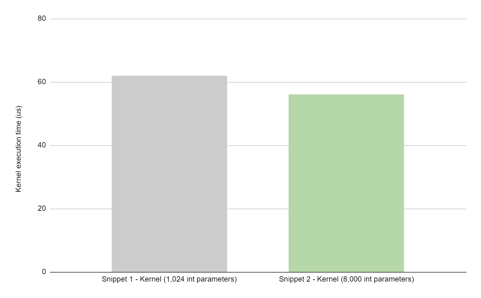
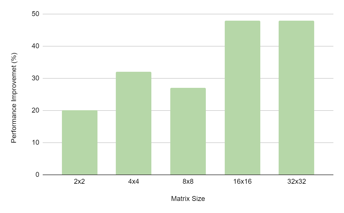
Figure 1 compares the performance of the two code snippets (provided above) on a single NVIDIA H100 system measured over 1,000 iterations. In this example, avoiding constant copies resulted in 28% overall savings in application runtime. For the same snippets, Figure 2 shows a 9% improvement in kernel execution time, as measured with NVIDIA Nsight Systems.
Figure 1. Application performance improvement with large kernel parameters on NVIDIA H100
For both images, the gray bar shows execution time for a kernel where 1,024 integers are passed as kernel parameters and remaining integers are passed using constant memory (code snippet 1). The green bar shows execution time for a kernel where 8,000 integers are passed as kernel parameters (code snippet 2). Both kernels accumulate 8,000 integers.
Figure 2. Kernel execution time improvement with large kernel parameters on NVIDIA H100
Note that if you omit the __grid_constant__ qualifier to the kernel parameter and perform a subsequent write operation to it from the kernel, an automatic copy to thread-local-memory is triggered. This may offset any performance gains.
Figure 3 shows the kernel execution time improvement profiled using Nsight Systems on QUDA. QUDA is an HPC library used for performing calculations in lattice quantum chromodynamics.
The reference kernel in this example performs a batched matrix multiply X * A + Y, where A, X, and Y are matrices. Kernel parameters store the coefficients of A. Prior to CUDA 12.1, when the coefficients exceeded the parameter limit of 4,096 bytes, they were explicitly copied over to constant memory, greatly increasing the kernel latency. With that copy removed, a significant performance improvement can be observed (Figure 3).
Figure 3. Kernel execution time improvement in QUDA with large kernel parameters
Summary
CUDA 12.1 offers you the option of passing up to 32,764 bytes using kernel parameters, which can be exploited to simplify applications as well as gain performance improvements. To see the full code sample referenced in this post, visit NVIDIA/cuda-samples on GitHub.
Jiusheng Chen’s team just got accelerated. They’re delivering personalized ads to users of Microsoft Bing with 7x throughput at reduced cost, thanks to NVIDIA Triton Inference Server running on NVIDIA A100 Tensor Core GPUs. It’s an amazing achievement for the principal software engineering manager and his crew. Tuning a Complex System Bing’s ad service uses Read article >
Editor’s note: This is part of a series profiling researchers advancing science with high performance computing. Maria Girone is expanding the world’s largest network of scientific computers with accelerated computing and AI. Since 2002, the Ph.D. in particle physics has worked on a grid of systems across 170 sites in more than 40 countries that Read article >
The NVIDIA Jetson Orin Nano and Jetson AGX Orin Developer Kits are now available at a discount for qualified students, educators, and researchers.Since its…
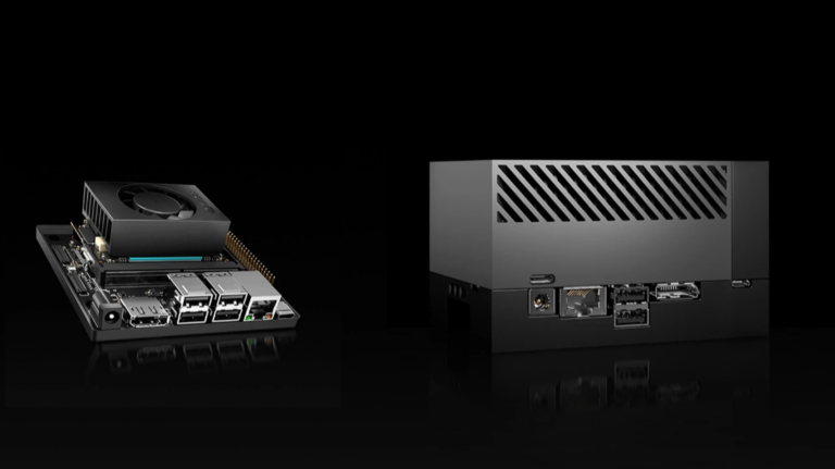
The NVIDIA Jetson Orin Nano and Jetson AGX Orin Developer Kits are now available at a discount for qualified students, educators, and researchers.Since its initial release almost 10 years ago, the NVIDIA Jetson platform has set the global standard for embedded computing and edge AI. These high-performance, low-power modules and developer kits for deep learning and computer vision give developers a small yet powerful platform to bring their robotics and edge AI vision to life. It’s the perfect tool for learning and teaching AI.
With 80x the performance over the original Jetson Nano, the Jetson Orin Nano Developer Kit enables you to run any kind of modern AI models, including transformer and advanced robotics models. It also has 5.4x the CUDA compute, 6.6x the CPU performance, and 50x the performance per watt compared to the Nano.
The NVIDIA Jetson AGX Orin Developer Kit and all Jetson Orin modules share one SoC architecture. This enables the developer kit to emulate any of the modules and makes it easy for you to start developing your next product. Compact size, lots of connectors, and up to 275 TOPS of AI performance make this developer kit perfect for prototyping advanced AI-powered robots and other edge AI devices.
The following videos show how easy it is to get started with the Jetson Orin Developer Kits.
Video 1. Getting Started with the Jetson Orin Nano Developer Kit
Video 2. Getting Started with the Jetson AGX Orin Developer Kit
Students making the most of Jetson developer kits
When you’ve got a Jetson-powered developer kit, imagine the possibilities for your next edge AI application.
For example, a group of mathematics, computer science, and biology researchers from the University of Marburg in Germany devised a way to quickly identify 80 species of birds and monitor local biodiversity based solely on the sounds those birds make. They used audio recordings captured with portable devices connected to the NVIDIA Jetson Nano Developer Kit.
Figure 1. Bird@Edge system built with the Jetson Nano
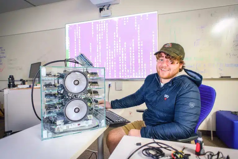
Last fall, students from Southern Methodist University in Dallas, built what they called a baby supercomputer using 16 NVIDIA Jetson Nano modules, four power supplies, more than 60 handmade wires, a network switch, and some cooling fans. Compared to a normal-sized supercomputer, which can be huge, this mini supercomputer fits neatly on a desk, enabling students to easily use it and learn hands-on.
Figure 2. SMU student with a baby supercomputer built using 16 Jetson Nano modules
Special student and educator pricing for Jetson Orin Developer Kits
If you are affiliated with an educational institution, you may be eligible for a discount on Jetson Orin Developer Kits. You must have a valid accredited university or education-related email address. You will then be provided with a one-time use code to order the Jetson Orin Nano Developer Kit or the Jetson AGX Orin Developer Kit. At this time, there is a limit of one of each kit per person.
Qualified students and educators can get the Jetson Orin Nano Developer Kit for $399 (USD) and the Jetson AGX Orin Developer Kit for $1,699 (USD). For more information, see Jetson for Education (login required). Requests for multiple units will be evaluated on a case-by-case basis.
The Ultimate School Supply: NVIDIA Jetson Nano
Figure 3. A Jetson Nano Developer Kit helps students get started
Don’t need all the power and performance from Jetson Orin? The NVIDIA Jetson Nano Developer Kit is the perfect companion for the upcoming back-to-school season. Powered by NVIDIA GPU-accelerated computing, the Jetson Nano brings your ideas to life, whether you’re a student, educator, or DIY enthusiast. From building intelligent robots to developing groundbreaking AI applications, the possibilities are endless.
Want to learn more about how you can use the Jetson Nano Developer Kit? Consider signing up for a free course from the NVIDIA Deep Learning Institute: Getting Started with AI on Jetson Nano. You may also want to look at the two Jetson AI certification programs available. For more inspiration, see the Jetson Community Projects page. Be sure to share your hard work in the Jetson forums so other developers can learn from your successes.
AI is transforming industries, automating processes, and opening new opportunities for innovation in the rapidly evolving technological landscape. As more…
AI is transforming industries, automating processes, and opening new opportunities for innovation in the rapidly evolving technological landscape. As more businesses recognize the value of incorporating AI into their operations, they face the challenge of implementing these technologies efficiently, effectively, and reliably.
Enter NVIDIA AI Enterprise, a comprehensive software suite designed to help organizations implement enterprise-ready AI, machine learning (ML), and data analytics at scale with security, reliability, API stability, and enterprise-grade support.
What is NVIDIA AI Enterprise?
Deploying AI solutions can be complex, requiring specialized hardware and software, as well as expert knowledge to develop and maintain these systems. NVIDIA AI Enterprise addresses these challenges by providing a complete ecosystem of tools, libraries, frameworks, and support services tailored for enterprise environments.
With GPU-accelerated computing capabilities, NVIDIA AI Enterprise enables enterprises to run AI workloads more efficiently, cost effectively, and at scale. NVIDIA AI Enterprise is built on top of the NVIDIA CUDA-X AI software stack, providing high-performance GPU-accelerated computing capabilities.
The suite includes:
VMI: A preconfigured virtual machine image that includes the necessary drivers and software to support GPU-accelerated AI workloads in the major clouds.
AI frameworks: Software that can run in a VMI (such as PyTorch, TensorFlow, RAPIDS, NVIDIA Triton with TensorRT and ONNX support, and more) that serves as the basis for AI development and deployment.
Pretrained models: Models that can be used as-is, or fine-tuned on enterprise-relevant data.
AI workflows: Prepackaged reference examples that illustrate how AI frameworks and pretrained models can be leveraged to build AI solutions to solve common business problems. These workflows provide guidance around fine-tuning pretrained models and AI model creation to build on NVIDIA frameworks. The pipelines to create applications are highlighted, as well as opinions on how to deploy customized applications and integrate them with various components typically found in enterprise environments, such as software for orchestration and management, storage, security, and networking. Available AI workflows include:
Intelligent virtual assistant: Engaging around-the-clock contact center assistance for lower operational costs.
Audio transcription: World-class, accurate transcripts based on GPU-optimized models.
Digital fingerprinting threat detection: Cybersecurity threat detection and alert prioritization to identify and act faster.
Next item prediction: Personalized product recommendations for increased customer engagement and retention.
Route optimization: Vehicle and robot routing optimization to reduce travel times and fuel costs.
Supported software with release branches
One of the main benefits of using the software available in NVIDIA AI Enterprise is that it is supported by NVIDIA with security and stability as guiding principles. NVIDIA AI Enterprise includes three release branches to cater to varying requirements across industries and use cases:
Latest Release Branch: Geared towards those needing top-of-the-tree software optimizations, this branch will have a monthly release cadence, ensuring users have access to the latest features and improvements. CVE patches, along with bug fixes, will also be included in roll-forward releases.
Production Release Branch: Designed for environments that prioritize API stability, this branch will receive monthly CVE patches and bug fixes, with two new branches introduced each year, each having a 9-month lifespan. To ensure seamless transitions and support, there will be a 3-month overlap period between two consecutive production branches. Production branches will be available in the second half of 2023.
Long-Term Release Branch: Tailored for highly regulated industries where long-term support is paramount, this branch will receive quarterly CVE patches and bug fixes and offers up to 3 years of support for a particular release. Complementing this long-term stability is a 6-month overlap period to ensure smooth transitions between versions, thus providing the longevity and consistency needed for these highly regulated industries.
Figure 1. The three release branches of NVIDIA AI Enterprise serve varying requirements across industries and use cases
How to use NVIDIA AI Enterprise with Microsoft Azure Machine Learning
Microsoft Azure Machine Learning is a platform for AI development in the cloud and on premises, including a service for training, experimentation, deploying, and monitoring models, as well as designing and constructing prompt flows for large language models. An open platform, Azure Machine Learning supports all popular machine learning frameworks and toolkits, including those from NVIDIA AI Enterprise.
This collaboration optimizes the experience of running NVIDIA AI software by integrating it with the Azure Machine Learning training and inference platform. Users no longer need to spend time setting up training environments, installing packages, writing training code, logging training metrics, and deploying models. With this integration, users will be able to leverage the power of NVIDIA enterprise-ready software, complementing Azure Machine Learning’s high performance and secure infrastructure, to build production-ready AI workflows.
To get started today, follow these steps:
1. Sign in to Microsoft Azure and launch Azure Machine Learning Studio.
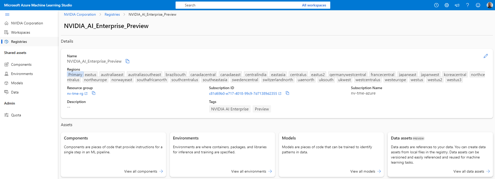
2. View and access all prebuilt NVIDIA AI Enterprise Components, Environments, and Models from the NVIDIA AI Enterprise Preview Registry (Figure 2).
Figure 2. NVIDIA AI Enterprise Preview Registry on Azure Machine Learning
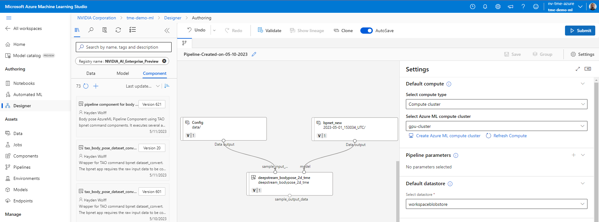
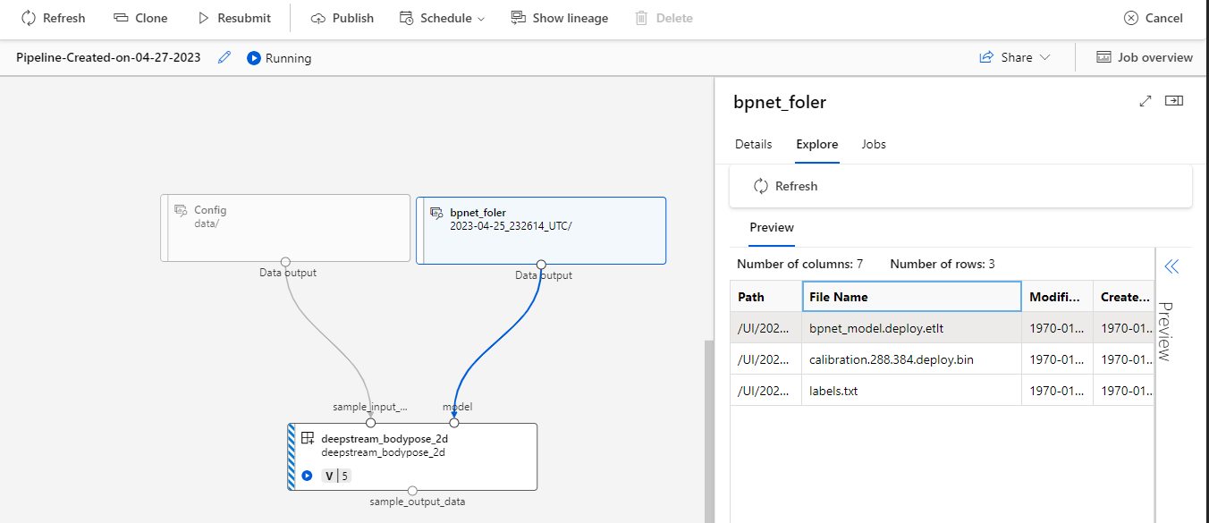
3. Use these assets from within a workspace to create ML pipelines within the designer through simple drag and drop (Figure 3).
Figure 3. Pipelines in Azure Machine Learning using NVIDIA AI Enterprise components
Find NVIDIA AI Enterprise sample assets in the Azure Machine Learning registry. Visit NVIDIA_AI_Enterprise_AzureML on GitHub to find code for the preview assets.
Use case: Body pose estimation
Using the various elements within the NVIDIA AI Enterprise Preview Registry is easy. This example showcases a computer vision task that uses NVIDIA DeepStream for body pose estimation. NVIDIA TAO Toolkit provides the basis for the body pose model and the ability to refine it with new data.
Figure 4 shows a video analytics pipeline example running the NVIDIA DeepStream sample app for body pose estimation. It runs on a GPU cluster and can be easily adapted to leverage updated models and videos, unlocking the power of the Azure Machine Learning platform.
Figure 4. NVIDIA TAO Toolkit and NVIDIA DeepStream for body pose estimation with Azure Machine Learning
The example includes two URI-based data assets created for storing the inputs for the DeepStream sample app command component. The data assets leverage a pretrained model, which is readily available in the NVIDIA AI Enterprise Registry. They also include additional calibration and label information.
The DeepStream body pose command component is configured to use Microsoft Azure blob storage. This component monitors the input directory for any new video files that require inference. When a video file appears, the component picks it up and performs body pose inference. The outputted video includes bounding boxes and tracking lines and is stored in an output directory.
Additional samples available within the registry include:
bodyposenet
citysemsegformer
dashcamnet
emotionnet
fpenet
gazenet
gesturenet
lprnet
peoplenet
peoplenet_transformer
peoplesemsegnet
reidentificationnet
retail_object_detection
retail_object_recognition
trafficcamnet
Each of these samples can be improved with a TAO Toolkit-based training pipeline, which performs transfer learning. The model output changes to fit a specific use case. You can find TAO Toolkit computer vision sample workflows on NGC.
Get started with NVIDIA AI Enterprise on Azure Machine Learning
NVIDIA AI Enterprise and Azure Machine Learning together create a powerful combination of GPU-accelerated computing and a comprehensive cloud-based machine learning platform, enabling businesses to develop and deploy AI models more efficiently. This synergy enables enterprises to harness the flexibility of cloud resources while leveraging the performance advantages of NVIDIA GPUs and software.
To get started with NVIDIA AI Enterprise on Azure Machine Learning, sign up for a Tech Preview. This will give you access to all of the prebuilt Components, Environments, and Models from the NVIDIA AI Enterprise Preview Registry on Azure Machine Learning.
When you see a context-relevant advertisement on a web page, it’s most likely content served by a Taboola data pipeline. As the leading content recommendation…
When you see a context-relevant advertisement on a web page, it’s most likely content served by a Taboola data pipeline. As the leading content recommendation company in the world, a big challenge for Taboola was the frequent need to scale Apache Spark CPU cluster capacity to address the constantly growing compute and storage requirements.
Data center capacity and hardware costs are always under pressure.
What caused the scaling challenges? Taboola uses a complex data pipeline stretching from user browsers or mobile devices through multiple data centers. Complex deep learning algorithms, databases, infrastructure services (such as Apache Kafka), and thousands of servers are deployed to serve the best-fitting ads to users around the world.
This post describes Taboola’s motivation to move to RAPIDS Accelerator for Apache Spark to optimize processing costs, along with insights on the migration process, challenges, and lessons learned to date.
Challenges of feeding a compute-hungry pipeline
To plan solutions, you must fully understand the magnitude of the problem. When serving ad content, Taboola builds a unique pageview that identifies each user and their interaction with the system. The pageview, a large, wide data structure, is built within a massive CPU cluster using data collected across worldwide data centers. The structure contains over 1500 distinct columns amounting to >1 TB of hourly data, all processed in our Apache Spark CPU cluster.
Many distinct analyzers and SQL queries process incoming pageviews at a rate of 1 TB of raw data per hour and catchup runs at 2, 6, 12, and 48 hours. New analyzers are constantly being created that increase the load on the Apache Spark cluster. There is a growing need for more compute power.
Our main task was to make the complex compute-hungry pipeline more scalable while being cost-effective. To address this challenge, Taboola embarked on an effort to migrate thousands of CPU cores to GPUs, to help us cope with the increasing data load to be processed.
One tool we considered to accelerate Taboola’s Apache Spark environments was the RAPIDS Accelerator on GPUs. As such, it was a natural decision to attempt greater scalability on GPUs as opposed to CPUs.
Key considerations
First, we defined what we needed for testing to successfully migrate thousands of CPU cores to leverage GPU acceleration:
Real-life dataset
Hardware specifications
Minimum X factor
Complex query testing
Real-life dataset
We used real production data from Cyber Monday to test and benchmark a large dataset. The data is 1.5 TB of ZSTD-compressed Parquet files per hour. It has over 1500 columns of all native types including arrays, structures, and nested structures with arrays.
Hardware specifications
For hardware, we started with the following resources:
A 72 CPU core Intel server with three A30 GPUs
A 900-GB local SSD drive, for Apache Spark to store its intermediate files
380 GB RAM
A 10-Gb/s NIC card
Minimum X factor
The primary question when migrating a project from the CPU to the GPU is usually, “What’s the X factor?” For a real-world cluster with multiple GPUs, the question is, “How many GPUs do I need for sustaining a load manageable by X CPU cores?” The answer is your X factor.
We set a minimum bar of an X factor of 3 for the GPU solution to be considered successful in terms of cost. This factor helps guarantee our migration efforts will pay off.
Complex query testing
We picked 15 queries from production across multiple R&D departments to resemble as many of the hundreds of queries as are in production.
The queries are mostly complex including many SQL operations:
Aggregations
Sorts
Lateral view explode
Distribute by
Window functions
UDFS
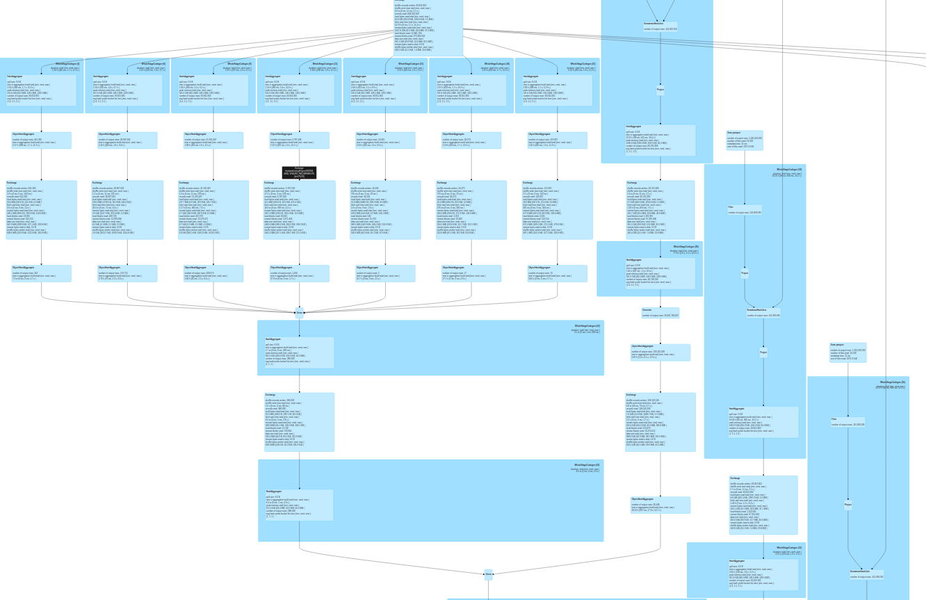
Figure 1 shows an example query.
Figure 1. Live sample of a large complex query in production requiring more compute power
Table 1 shows you Taboola’s factors.
Analyzer name
Avg CPU production time
Avg GPU time
GPU factor
AdvertiserDimensionByRequest
586.41
31.91
18.38
ExperiementAnalysisPage
3021.6
102.92
29.36
ExperiementAnalysisPlacement
680.84
47.12
14.45
ExperimentAnalysisRequestBase
6605.44
362.68
18.21
ExperimentAnalysisSession
207.87
23.01
9.03
MediaDatatrendsBase
222.94
9.8
22.75
PerformanceMeasurements
397.17
86.22
4.61
PublisherPerformance
965.63
108.95
8.86
RBoxABTest
63.04
2.4
23.88
RevenueByHostHourly
487.44
95.03
5.13
SlaUnitAvailableFillRate
1199.93
152.38
7.87
SupplyDataTrends
529.92
45.28
11.7
Table 1. Production speedups
CPU-to-GPU migration goals
We began with a single server (as described earlier) capable of scaling to a multi-GPU and multi-server cluster. The cluster would be managed by Kubernetes, as opposed to the current Mesos cluster. Mesos was going to become obsolete and NVIDIA environments support Kubernetes.
Any changes in the software and hardware environment would have to be oblivious to Taboola’s code. Queries run on GPUs should execute with the exact results as CPUs. The team was aware of this challenge, as production stability was a critical goal.
Lastly, we wanted the GPU to outperform the CPUs by a minimum factor of 3. We benchmarked several GPUs including NVIDIA P100, NVIDIA V100, NVIDIA A100, and NVIDIA A30. We learned that the A30 GPU gave us the best price-performance fit.
First experiment with RAPIDS Accelerator
We ran SQL queries using RAPIDS Accelerator with somewhat disappointing results. Some of the less complex queries, mostly with lateral view explode, gave a 3x to 5x factor over the CPU. Some showed much lower factors, while other queries crashed.
After asking questions in the RAPIDS GitHub repo, we tried relevant Apache Spark and RAPIDS Accelerator parameters and began seeing better results:
sql.files.maxPartitionBytes: The CPU uses a default value of 128 MB. This is too low for the GPU. We are using 1–2 GB.
sql.shuffle.partitions: We found the 200 default to be sufficient in most cases.
rapids.sql.concurrentGpuTasks: Determines the number of tasks that can be run concurrently on the GPU. A minimum of at least two tasks appears to be best.
Tuning these parameters helped the queries run more smoothly and perform better in some cases. The NVIDIA Accelerated Spark Analysis tool can automatically generate tuning recommendations.
Challenge #1 – Parquet parsing overhead
We experienced bottlenecks on some of the less performant SQL queries, with most of them wasting time parsing Parquet footer data on the CPU. The Parquet data has more than 1500 columns. It was apparent that regular Java code for parsing the footer was not adequate for such a large footer.
Figure 2 shows a small section of NVIDIA profiler output for a 9-second Apache Spark task where the GPU was mostly idle (only working for 330 ms).
Figure 2. Inefficient Parquet parsing trace
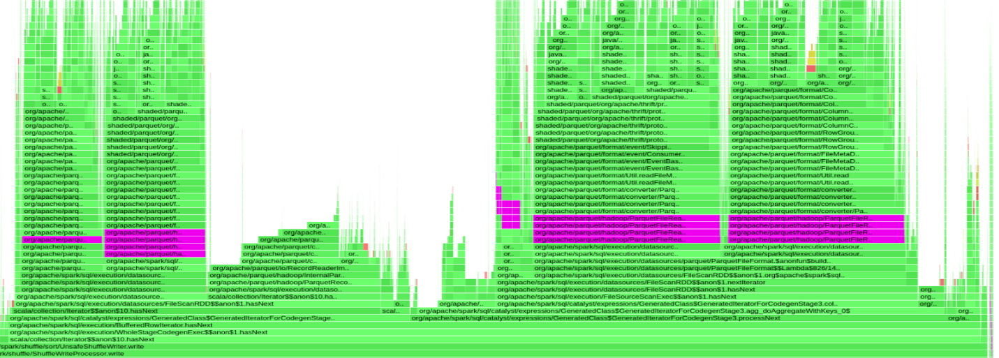
Figure 3 shows a flame graph of a query suffering from this behavior. The purple bars indicate time spent inside the org.apache.parquet.hadoop.ParquetFileReader class. Almost 50% of the query time was spent on parsing Parquet’s footer while the GPU was idle.
Figure 3. Trace showing inefficient Parquet parsing in purple bars
As such, we set off to test an alternative solution. When parsing the footer, Parquet code would iterate over footer metadata serially for each row group. We adjusted Parquet parameters to decrease the number of row groups in each file. This gave us about 10–15% improvement. We found this improvement to be insufficient.
Each time metadata was read, all 1500 columns of metadata were read and parsed serially, even after only asking for 50-100 columns per query. We wanted to index footer metadata such that instead of reading the entire 1500 data columns serially, we’d just access it directly. We managed to make this happen by changing the Parquet-mr public code in C++ and Java. Although we got nice performance results, this was too cumbersome and complex.
Fortunately, the NVIDIA RAPIDS team had a much better idea. The solution was optimal Parquet file parsing. They replaced the Java code with Arrow’s C++ implementation. We now have the rapids.sql.format.parquet.reader.footer.typeset to NATIVE by default for our GPU implementation. The bottleneck was solved and there were no longer queries with the GPU idle because of footer parsing overheads on the CPU.
Challenge #2 – Network bottleneck
A weak network card caused the next bottleneck. While the 10-Gb/s Ethernet card sustained the CPU load, it failed to do so for the GPU load.
The solution was an optimal network card for GPU loads. Replacing the 10-Gb/s Ethernet card with a 25-Gb/s card removed this bottleneck.
Challenge #3 – Disk I/O bottleneck
Even after removing the two bottlenecks, queries still ran slow. On the Apache Spark user interface, we saw a clear indication as to what was happening.
Metric
Min
25th percentile
Median
75th percentile
Max
Duration
0.4 s
0.6 s
0.8 s
1 s
1.2 min
GC Time
0.0 ms
0.0 ms
0.0 ms
90.0 ms
0.5 s
Shuffle Read Size/Records
21.4 MB/1000
22.3 MB/1000
22.5 MB/1000
22.7 MB/1000
27.3 MB/1000
Shuffle Write Size/Records
17.5 MB/1000
17.9 MB/1000
18 MB/1000
18.1 MB/1000
18.1 MB/1000
Scheduler Delay
3.0 ms
5.0 ms
5.0 ms
7.0 ms
3 s
Peak Execution Memory
64 MB
64 MB
64 MB
64 MB
64 MB
Shuffle Write Time
9.0 ms
13.0 ms
18.0 ms
21.0 ms
59 s
Table 2. Statistics of disk I/O bottlenecks
In Table 2, in the Max column, the task’s duration is 1.2 minutes, while Shuffle Write Time took 58 seconds. A lot of time was wasted doing shuffle work while the GPU was idle.
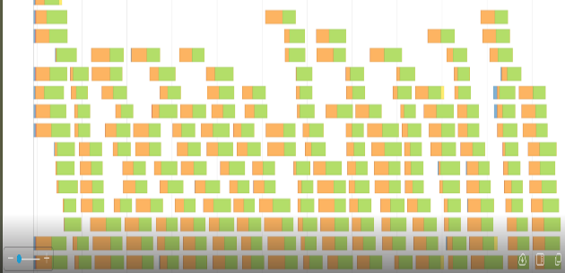
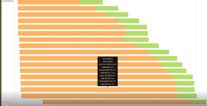
Figures 4 and 5 show the appropriate event timeline graph. The orange part represents shuffle times, read or write. The green parts are compute time. We were wasting a lot of time reading or writing shuffle files.
Figure 4. Event timeline graph of Disk I/O bottlenecks as segments
Figure 5. Event timeline bar chart of disk I/O bottlenecks
Our shuffle files can get up to 500 GB and greater in some queries. We obviously can’t keep this huge amount of data in the server’s RAM, so shuffle files are stored in the local SSD drive.
After a quick investigation with our teams, we figured out that the SSD drive was configured to use RAID-1. Each temporary shuffle file was saved twice to the disk. This wasted a lot of time and switching to RAID-0 somewhat improved the situation.
The GPU put more pressure on the SSD drive than the CPU such that we had to replace the SSD with an NVMe drive. The solution was to switch to a 6-TB NVMe drive. We removed one of the GPUs to create a slot for the NVMe drive. Afterward, we had no shuffle read or write performance issues. We also learned that one NVMe drive could sustain the workload of two A30 GPUs.
Moving to Kubernetes
Because our Mesos cluster would become obsolete, the move to Kubernetes from a standalone POC machine was imperative. This involved a lot of configuration work, and other minor work. Still, it was straightforward to implement.
The basic idea is that the Apache Spark driver would sit on a non-GPU machine and each K8s Pod would be associated with a single GPU. For more information, see Getting Started with RAPIDS and Kubernetes.
The following code example shows some of the major relevant Kubernetes configurations.
If the goal is to use GPUs to accelerate workloads more cost-effectively than CPUs, we first had to understand how fast GPUs were. We set up a test system with two A30 GPUs and streamed production data to it in parallel with our large CPU core production environment.
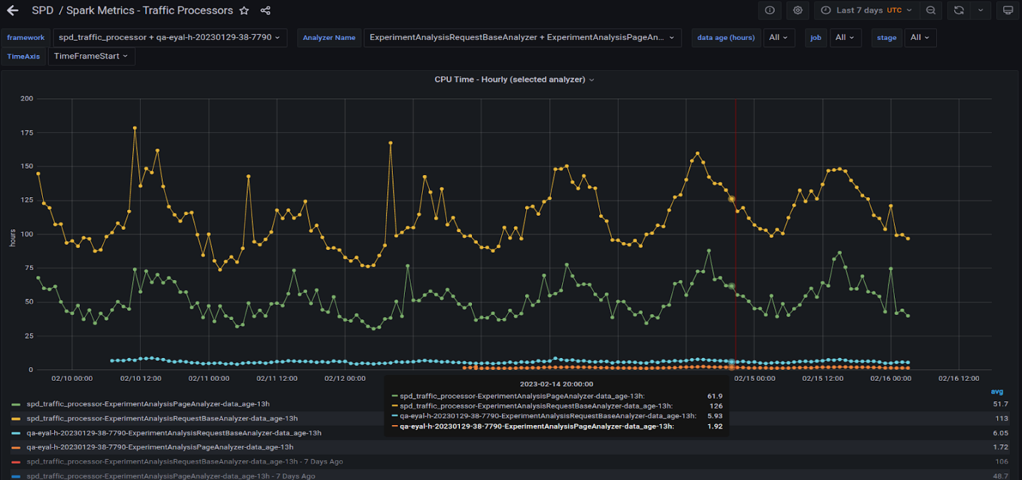
Figure 6 shows two of our heaviest queries running on the production CPU cluster and also on the server with two A30 GPUs.
Figure 6. Heavy queries and resulting hourly processing time for CPU and GPU
The yellow and green lines denote the hourly total time across all task numbers of the two queries running on the CPU cluster. The blue and orange lines denote the same queries running on the GPU server. GPU factors are 20x and higher.
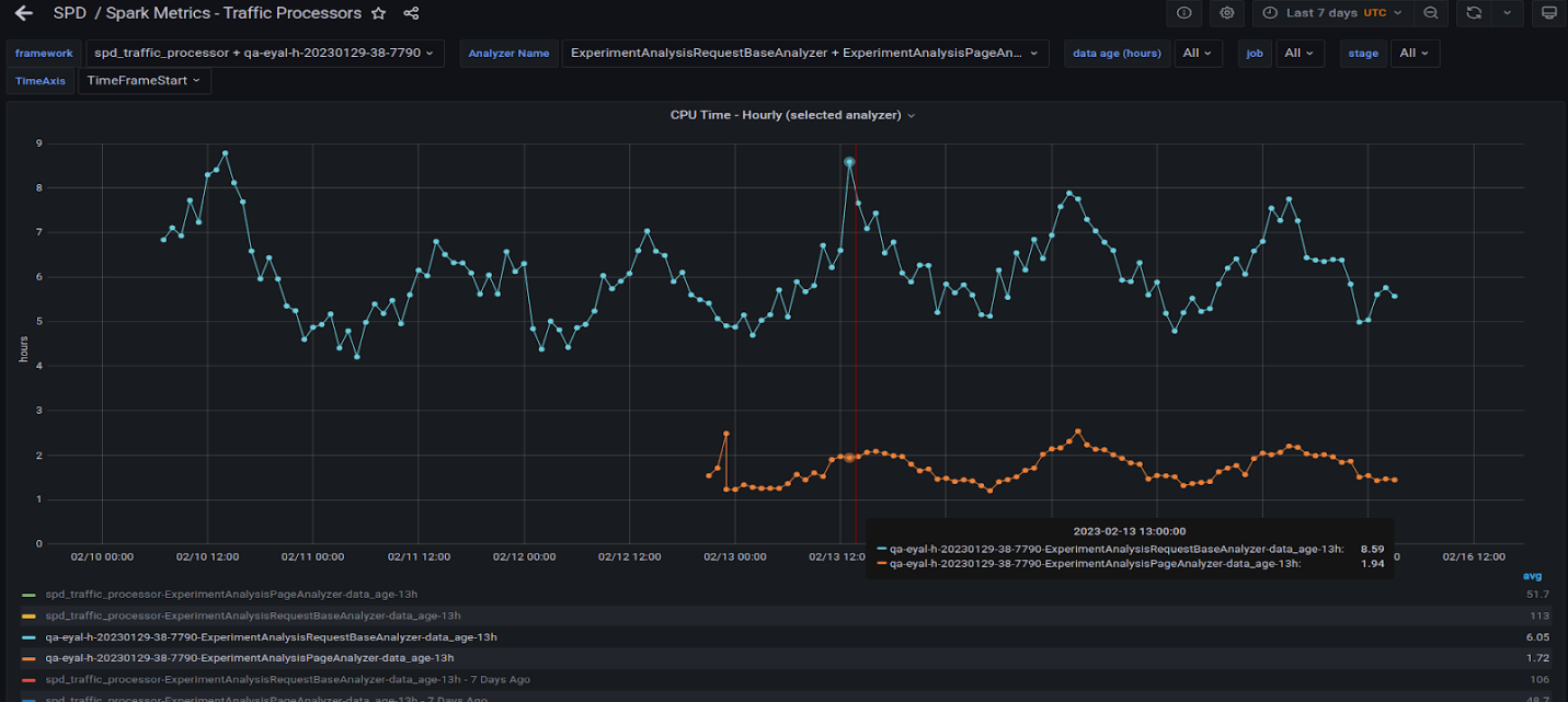
Figure 7 shows the two queries running on the GPU shown in Figure 6. Observe that they behave similarly to the CPU in that peaks and valleys roughly align at different times of the day.
Figure 7. Hourly GPU total time across all tasks
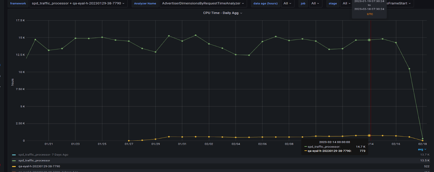
Figure 8 is interesting in that it shows the factor of all the queries that we migrated to the GPU and their counterparts on the CPU. The GPU run is missing the biggest query, which we are still working on migrating to the GPU. It will likely add 200 hours per day to the GPU total time.
Figure 8. Daily aggregation comparison of CPU vs GPU times
Lessons learned
Looking ahead to our next migration steps, Taboola would like to move queries from other R&D departments to the GPU, resulting in a greater number of GPUs in production. This means that QA must monitor the system more closely while in production.
Getting acquainted with RAPIDS Accelerator for Apache Spark was an amazing “joy ride” effort. From handling Parquet files to pushing GPUs to their limit, we became better equipped at handling a large data pipeline along with managing data center capacity and hardware costs. Identifying and coping with hardware limitations with this method proved to be rewarding.
Here are Taboola’s top takeaways for those considering CPU-to-GPU migration:
Tuning parameters in complex environments that have multiple variables is never straightforward. Automate this task to whatever degree possible. It’s probably a good idea to use the NVIDIA Accelerated Spark Analysis tool to help address this challenge, as it can easily suggest optimized parameters.
Look beyond CPUs and GPUs for solutions to bottlenecks. No amount of GPU horsepower can resolve issues that are fundamentally network, disk, bandwidth, or configuration and parsing related.
Multiple GPUs do not hinder performance, but GPUs are so powerful that you may have good performance with fewer GPUs than originally thought. It’s best to test for this to lower costs.
We achieved our 20x factor through RAPIDS Accelerator and NVIDIA GPUs. The biggest lesson learned was that we needed to better understand what was happening in our existing environment before benefiting from GPU acceleration. One A30 GPU sustained the same production load for some workloads as the ~200-CPU core test cluster.
For more information about achieving performance multiples over Apache Spark CPU-based environments, see GPU-Accelerated Apache Spark.
Acknowledgments
Our huge effort was more successful with the support, assistance, and patience of two great groups of people. At Taboola: Andrey Gourine, Gilad Zamoscinski, Igor Berman, Keren Corsia, Lior Chaga, and Michael Taranov. On the NVIDIA RAPIDS team: Alessandro Bellina, Hao Zhu, Karthikeyan Rajendran, Robert Evans, and Sameer Raheja.

 NVIDIA Modulus is a framework for building, training, and fine-tuning deep learning models for physical systems, otherwise known as physics-informed machine…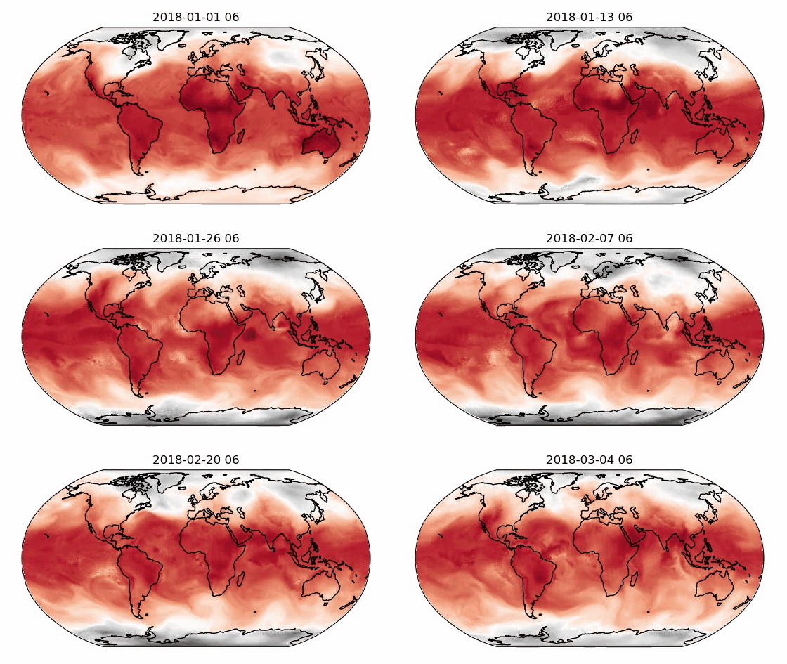
 Voice-enabled technology is becoming ubiquitous. But many are being left behind by an anglocentric and demographically biased algorithmic world. Mozilla Common…
 CUDA kernel function parameters are passed to the device through constant memory and have been limited to 4,096 bytes. CUDA 12.1 increases this parameter limit…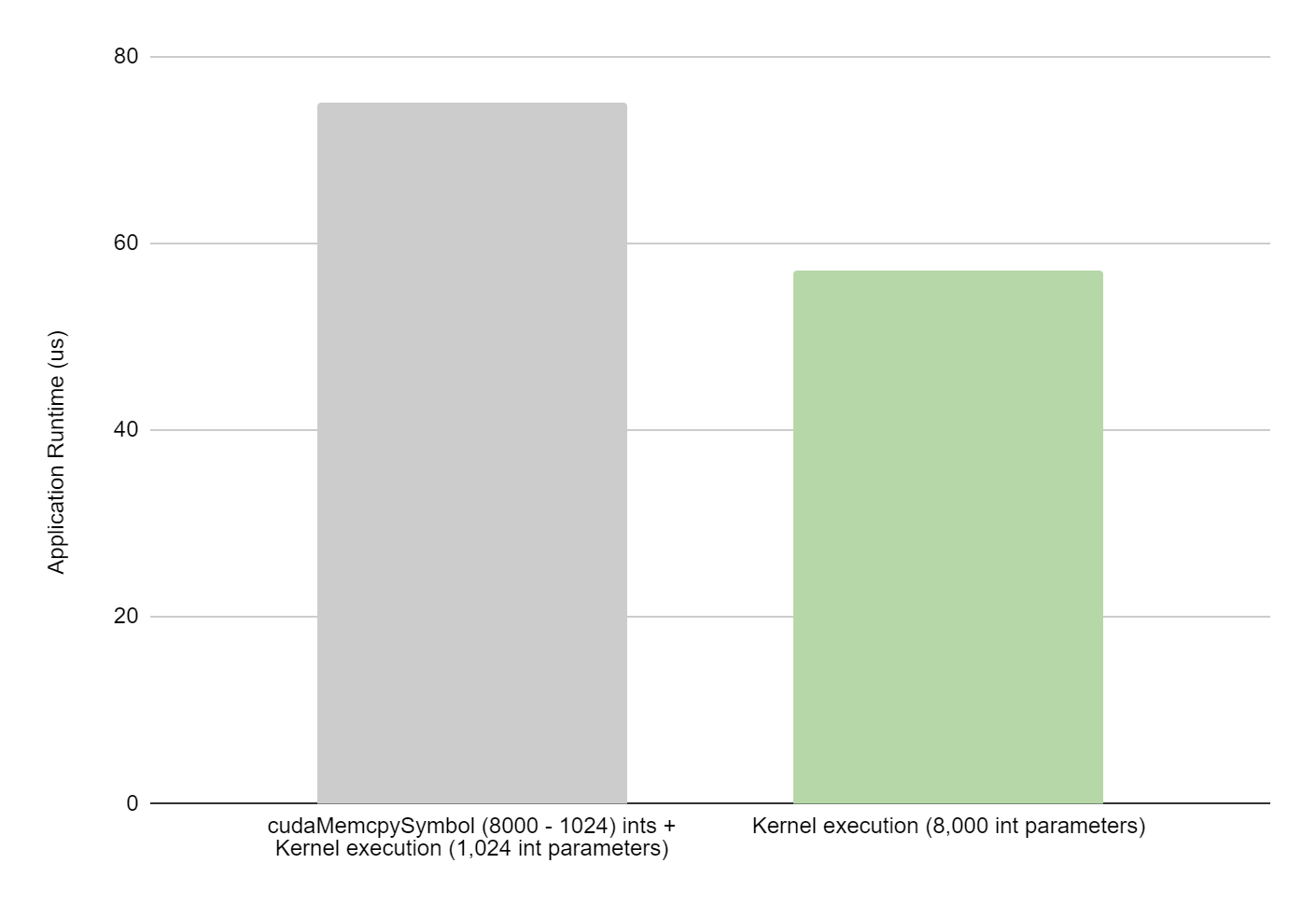
 The NVIDIA Jetson Orin Nano and Jetson AGX Orin Developer Kits are now available at a discount for qualified students, educators, and researchers.Since its…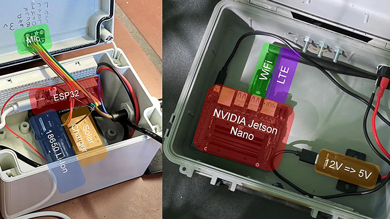

 AI is transforming industries, automating processes, and opening new opportunities for innovation in the rapidly evolving technological landscape. As more…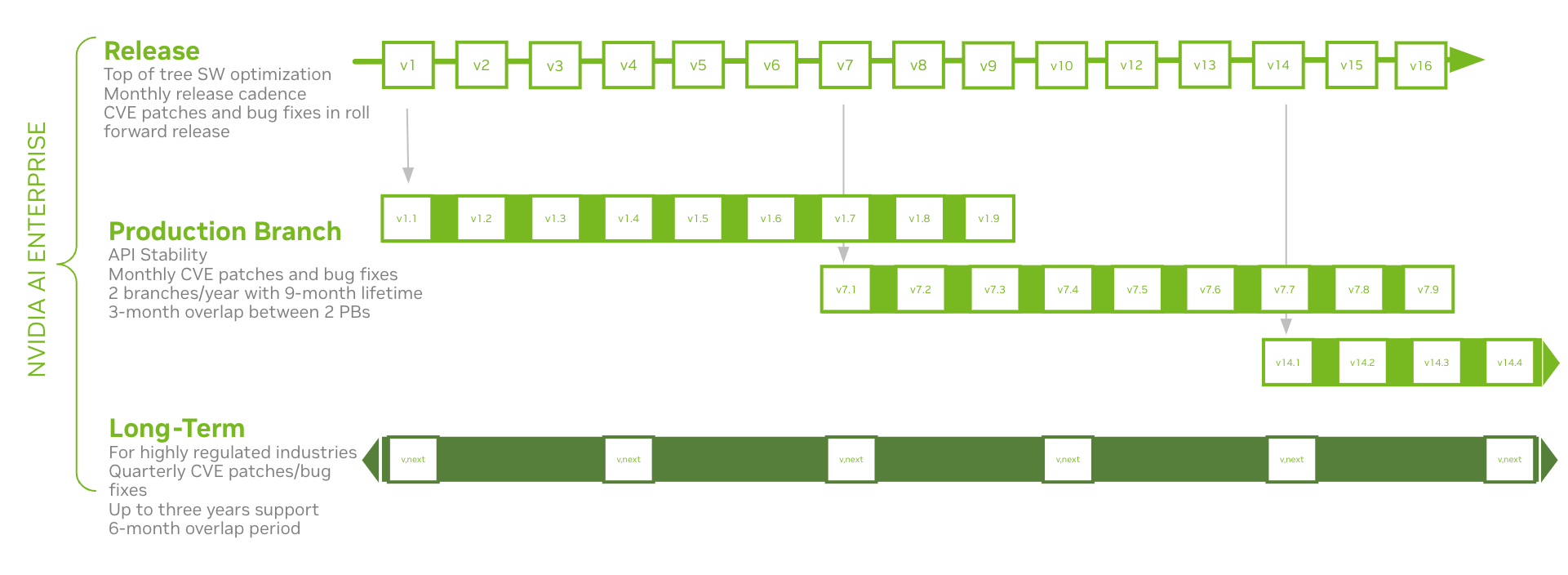
 When you see a context-relevant advertisement on a web page, it’s most likely content served by a Taboola data pipeline. As the leading content recommendation…