I am getting the same prediction for different inputs. I am trying to use a regressional neural network. Since data is huge, I am training one example at a time. Here is a simplified version of my code.
model = Sequential() model.add(Dense(10000, input_dim=212207, kernel_initializer='normal', activation='relu')) model.add(Dense(100, activation='relu')) model.add(Dense(1, kernel_initializer='normal')) model.compile(loss='mean_squared_error', optimizer='adam') for i in range(10000000): #X is input with 212207 values #Y is a output value if i<6000000: model.fit(X.transpose(), Y, epochs=30, batch_size=1, verbose=0) else: prediction=model.predict(X.transpose())
I made sure that I am training on different examples and trying predictions on different examples. I am still getting the same prediction value for all testing inputs. I think I made some mistake in defining the model for regression neural network. Can you please check if the code is correct?
Is there an ideal network design that always works? Let’s find out. This blog covers the pros and cons of pure layer 3, layer 2 only, and VXLAN and EVPN.
Network administrators have a hard job. They are responsible for ensuring connectivity for all users, servers, and applications on their networks. They are often tasked with building a network design before getting application requirements, making a challenging project even more difficult. In these scenarios, it’s logical for networking admins to try to find an ideal network design they can use with any set of applications.
There is no one-size-fits-all network solution that will work every time, and every design has benefits and drawbacks. In this post, we analyze three different network types that could be perceived as ideal. Then, we describe where each falls short, based on real-world factors.
The candidates are:
Pure layer 3
Layer 2 only
Overlay with VXLAN and EVPN
Ready? Let’s get started.
Pure layer 3 design
Many forward-thinking architects think pure layer 3 (L3) is the ideal design due to its simplicity and reliance on only one protocol stack. All traffic is routed and balanced at the L3 level using equal-cost multipath and endpoint redundancy is achieved through a natively functional anycast address solution. It’s simple and elegant.
Many large web-scale IT companies choose it for its excellent operational efficiency. It also gives them robust control over their application environment to design applications that work within this design.
Applications that rely on network overlays or pure routing are optimized for the L3 architecture. Whether using a container-based solution that leverages routing as its mechanism to provide access to the environment, or a Container Network Interface to encapsulate the container-to-container communication, these solutions work great on this architecture.
The advent of SmartNICs and DPUs makes L3 more user-friendly by providing host-based solutions to offload resource-intensive tasks such as storing routing tables, performing packet encapsulation, and doing NAT.
The biggest drawback with L3 is that it doesn’t allow any distribution of layer 2 (L2) adjacency. Over time, most enterprises must introduce an application that requires L2 adjacency, either within or between racks. Historically, developers have been unreliable in writing their applications to handle clustering using L3 capabilities. Instead of using DNS or other L3 discovery processes, many legacy applications use L2 broadcast domains to discover and detect nodes to join the cluster. A pure L3 solution struggles to service software that requires such an environment because each L2 domain is limited to one node or one server.
Layer 2 only design
The L2 only solution is the opposite of pure L3. L2 only primarily leverages VLANs for segregating its connectivity and relies on legacy features like MLAG and spanning tree protocol (STP) to provide a distributed solution. The L2-only solution still has a place in network environments, typically in simple, static environments that don’t require scale.
People are comfortable with L2, as it uses tried-and-true technologies familiar to most people. It’s simple in the protocol stack, making all forwarding decisions based on only the first two layers of the OSI model. Also, most low-cost network devices on the market are capable of these feature sets.
However, L2 has gaps in scale and performance. Relying on STP across three tiers to prevent loops, leads to inefficient redundant paths. To circumvent this limitation in spanning-tree convergence, you can try deploying back-to-back MLAG. MLAG is not as efficient as a pure layer 3 solution at handling device failures and synchronizing control planes, however. L2 networks tend to limit broadcast and multicast traffic. These are just a few limitations that create a hidden cost of ownership around deploying an L2 only design.
Overlay design: VXLAN and EVPN
The most common design in the enterprise data center is VXLAN as the transport layer encapsulation technology, with EVPN as the control plane technology. This architecture provides the greatest flexibility, with all the benefits of a pure layer 3 solution, and provides the network administrator the adaptability to support applications requiring L2 to function.
It provides the benefits of L2 adjacency without introducing inefficient protocols such as STP and MLAG. Leveraging EVPN as the L2 control plane and multihoming as the optimal alternative to MLAG, overlay solutions solve many inefficiencies with L2.
A one-size-fits-all solution like VXLAN and EVPN could be thought of as ideal, but even this has drawbacks. Its detractors point to the multiple layered protocols required to make it operate. The solution builds on a BGP-enabled underlay with EVPN configured between the tunnel endpoints. VXLAN tunnels are configured on top of the overlay with varying levels of complexity depending on tenancy requirements. This may include integrating with VRFs, introducing L3 VNIs for intersubnet communication, and the reliance on border leafs for intertenant communication through VRF route leaking. Combining all these technologies can create a level of complexity that makes troubleshooting and operations difficult.
Conclusion
Everything has tradeoffs, whether you’re sacrificing operational complexity for network simplicity or trading application control for flexibility. The upside of accepting that there is no perfect network design is that you are now free to pick and choose the architectures and workflow that best fit your network. Work with your application and infrastructure teams to identify the server requirements, optimize your workflows, and select the best solutions for your applications’ needs.
To scale AI for financial services, companies must face several resource hurdles. The full-stack solution from NVIDIA and VMware helps you leverage the competitive advantages of AI.
AI adoption has grown rapidly over the past few years due to its ability to automate repetitive tasks and increase revenue opportunities. Yet many companies still struggle with how to meaningfully scale AI in financial services. Increased data needs and a lack of internal talent are a few issues.
In this post, we provide a landscape overview of AI use cases and highlight some key scaling challenges, along with how leading banks and financial institutions are using end-to-end solutions to mobilize AI adoption.
What drives the use of AI in financial services?
The power of AI to solve complex business problems is widely recognized in the financial services industry, an early adopter of data science. Banking is among the top three industries in annual investment in big data and analytics. An NVIDIA survey found that 83% of C-suite leaders, IT architects, and developers in financial institutions believe that AI is vital to their future success.
It is easy to understand why: Business Insider estimates that the potential for AI-driven cost savings for banks will reach $447 billion by 2023. Across consumer finance and capital market sectors, firms are looking for ways to mine that potential.
Improved fraud detection and prevention rank highest among proven AI use cases, especially with online-payment fraud losses expected to hit $48 billion annually by 2023.
Other business drivers include maximizing client returns through portfolio optimization or creating personalized customer service through call center transcription. The list continues to grow.
A recent paper by McKinsey and Company underscores the coming sea change: to thrive, banks need to operate “AI first.” Therefore, realizing AI’s value does not come from single projects or teams but instead requires collaboration among data engineers, data scientists, and app developers across the financial institution, all supported by an AI-enabled IT infrastructure.
Finance industry use cases
The quickest returns often stem from improved fraud detection and prevention, the most cited use of AI in financial services. AI is also beneficial for creating efficiencies and reducing compliance costs related to anti-money laundering efforts and know-your-customer regulations.
When combining risk management with profit maximization, investment firms increasingly look to AI for building algorithmic trading systems, which are powered by advances in GPUs and cloud computing. Analysts involved in asset management and portfolio optimization can use natural language processing (NLP) to extract more relevant information from unstructured data faster than ever before, reducing the need for labor-intensive research.
Within consumer finance, NLP helps retail banks gain a better understanding of customer needs and identify new marketing opportunities through call center transcription. Along with chatbots and virtual assistants, transcription falls within the larger category of conversational AI, which helps personalize service by creating 360o views of customers.
Another use of AI within customer engagement is recommendation engines. This technology improves cross-selling by leveraging credit usage, scoring, and balances to suggest fitting financial products.
Key challenges of scaling AI
Banking, trading, and online-payment firms that do not adopt AI and machine learning (ML) risk being left behind, but even companies that embrace the technology face hurdles. In fact, almost half of AI projects never make it to production.
Elevated costs
One fundamental concern: AI demands exceed the existing IT infrastructure for most companies. The tooling that data scientists require for AI workloads is often difficult to deploy onto legacy systems. 28% of IT pros rate the lack of infrastructure as the primary obstacle to adoption. The proliferation of AI apps is also making IT management increasingly difficult.
Shadow IT
Financial institutions that invest in AI only within a research lab, innovation team, or line of businesses frequently have data scientists operating on customized bare-metal infrastructure. This setup produces silos in data centers and leads to shadow IT existing outside departmental IT control.
These silos further hinder productivity. Rather than focusing on training ML models, data scientists spend more time as de facto IT managers for their AI fiefdoms.
Furthermore, if that infrastructure does not include accelerated computing and the parallel processing power of GPUs, deep learning models can take days or weeks to train, thereby wasting precious time for data scientists. It is like hiring world-class race car drivers and equipping them with Yugos.
Unused infrastructure
As expected, costs begin to spiral. Disparate IT increases operational overhead. Inefficient utilization of infrastructure from silos results in higher costs per workload when compared with the cloudlike efficiency achieved by allocating resources on demand through virtualization. Expensive data scientists are forced to manage IT, and ROI slows. AI projects languish.
AI-driven platforms offered by NVIDIA and VMware
So how can financial institutions fully adopt AI, scale what they have implemented, and maximize its value?
Built on NVIDIA GPUs and VMware’s vSphere with Tanzu, NVIDIA AI Enterprise offers an end-to-end platform with a suite of data science tools and frameworks to support diverse AI applications. Crucially, it also helps reduce time to ROI while overcoming problems posed by ad hoc implementations.
NVIDIA and VMware’s full-stack solution is interoperable from the hardware to the application layer, providing a single platform for both financial services apps and AI workloads. It eliminates separate AI infrastructure, as it is developed on common NVIDIA-Certified Systems with NVIDIA GPUs and VMware vSphere with Tanzu, a cloud computing platform that already exists in most data centers.
This enterprise suite offers the AI tooling of TensorFlow, PyTorch, and RAPIDS, while vSphere’s Tanzu Kubernetes Grid can run containerized apps orchestrated with Kubernetes alongside virtualized apps, creating consistent infrastructure across all apps and AI-enabled workloads.
That consistency pulls data science out of silos and brings deployment into the mainstream data center, joining the IT team with data scientists and developers. Expensive devices like GPUs and accelerators can be shared using NVIDIA virtual GPUs, driving down the total cost of ownership while providing the speed-up needed to train ML models quickly. Meanwhile, data scientists are freed from IT management to focus on their specialized work.
In other words, IT leads get simplicity, manageability, easy scaling, and deployment; data scientists are supported with infrastructure and tooling that facilitates their core work; and business executives see quicker and greater ROI.
Summary
These applications merely scratch the surface of what is possible with AI in financial services, especially as the technology matures. To scale AI for financial services, companies can increase resource capacity, hire domain-specific expertise, and find innovative ways to govern their data.
The full-stack solution from NVIDIA and VMware provides a platform to leverage the competitive advantages of AI across entire firms while overcoming common implementation challenges.
See what the platform can do for you with immediate trial access to the NVIDIA AI Enterprise software suite LaunchPad, which runs on private accelerated computing infrastructure in VMware vSphere environments and includes a curated set of hands-on labs for AI practitioners and IT staff.
3D Artist Daniel Martinger discusses how he captured the attention of the computer graphics world with a path-traced rendered scene using an NVIDIA RTX 3090 and Unreal Engine 5.
NVIDIA was fortunate enough to speak with 3D prop and environment artist Daniel Martinger, who captured the attention of the computer graphics world with his stunningly realistic path-traced rendered scene entitled “The Carpenter’s Cellar.”
Below, Martinger discusses how he created this piece of work using an NVIDIA RTX 3090 and Unreal Engine 5, along with where he finds inspiration.
Figure 1. Fully path-traced scene in Unreal Engine 5.
Where do you look for inspiration and ideas? Martinger: Before I start a project, I really need to have a clear vision and an idea in my mind. I need to feel very excited to start the project. When I am outside, I often observe objects around me in nature and how lightning affects them. For example, during the day when I am outside or inside watching a movie—I get ideas of an environment and want to recreate it in 3D.
My ideas come from my surroundings. If I watch a movie and I see something cool that interests me like a messy room, I start to google reference photos of similar rooms. If I like the feeling of the room, there’s the possibility of combining that feeling with another theme. In this case I spent time searching for cellar reference photos like old cellars, just to get a feeling for the project.
Google and Pinterest are really nice sources. I gathered my references on a mood board. I usually have a lot of references just to combine them visually in my mind. In this project I really wanted daylight to spread throughout the room and explore Unreal Engine’s new lightning tech.
Why did you choose Unreal Engine 5 for this project? Martinger: In school we learned another game engine, and I am always looking to learn and update my skills. I also saw a lot of videos about Unreal Engine 5 and was very impressed, so I decided to use Unreal Engines’ new tech to present my art.
I have leveraged NVIDIA GPUs since I was 15. When the [RTX] 3090 came out, it was like a 3D artist’s dream. The VRAM plays a big role here compared to other cards. You can never have enough VRAM as a 3D artist!
The power of the 3090 is amazing. Texturing programs and the game engine, it all just works, there’s been no lag or stuttering. My computer didn’t “complain” much, I can work with 8k textures without any problems.
Did you incorporate any DXR features? Martinger: Yes, I enabled DX12 and I decided to go with full path tracing for the scene. I know I had to enable DirectX 12 for the path tracer and hardware ray tracing to be able to use path tracing, I played around with some ray tracing stuff in post effects like global illumination, ray tracing, and reflections, but I only used the path tracer for rendering images and videos. I played around with the real-time features, but it didn’t give me the quality of the path tracer.
How did you feel about the visual comparison between the Unreal Engine 5 path tracer versus offline renderers or other engines you’ve used? Martinger: I haven’t used many other offline renderers, but I have seen a lot of art created in Arnold. It feels like path tracing in Unreal Engine is very similar to Arnold. In Unreal Engine 5 the path-tracing feature is very user friendly. This is the first time I used an offline renderer, so I don’t have much to compare it with. I have only worked with one other game engine before Unreal Engine. Even without path tracing I think Unreal Engine is a very powerful engine for artists and can achieve amazing realistic results.
Are you using one or two light sources in the path traced render? Martinger: I wanted daylight to come into the room, so I used a skylight and a directional light as the sun source. I tweaked the settings to achieve the look I wanted, and yeah, path tracing just works. In real time you need to do a lot more work and tweaking to get a similar look as path tracing.
What are your biggest takeaways from this project? Martinger: Keeping a realistic goal and timeline in mind is key. Do something you can deliver in a reasonable amount of time, and most importantly detailed planning to map out the approach, project flow, and process.
I show how NVIDIA Isaac Sim and NVIDIA Isaac ROS GEMs can be used with the Nav2 navigation stack for robotic navigation.
NVIDIA Isaac ROS GEMs are ROS packages that optimize AI-based robotics applications to run on NVIDIA GPUs and the Jetson platform. There is a growing interest in integrating these packages with the Nav2 project to help autonomous robots successfully navigate around dynamic environments.
This work is done entirely in simulation and can be used as a starting point for transferring robotic capabilities from simulation to the real world (Sim2Real).
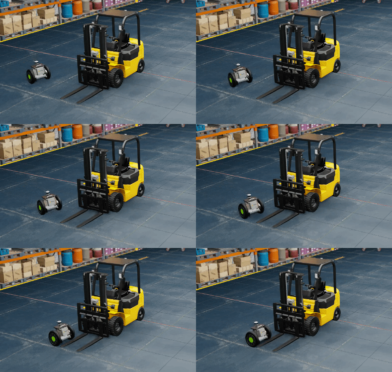
In this post, I focus on a real-world problem where robots are damaged due to collisions with forklift tines in warehouses. A forklift is an industrial truck used to move heavy objects over short distances. It has extensions called tines (or forks), which slide under and lift objects.
Figure 1. Forklifts
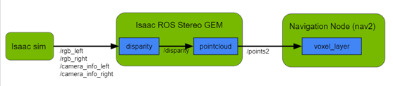
Primarily used robot sensors (lidar) can detect the body of a forklift, but not the tines, which are close to the ground. There is also a need for other sensors in this scenario that can detect these tines. In this project, you use two RGB cameras on the robot in simulation. The images from these cameras are used to calculate disparity using the Isaac ROS stereo GEM.
From disparity, the stereo GEM generates a point cloud, which contains information about where all the objects that are in the cameras’ field of view are in the environment. This information is used to update the navigation node such that the robot’s path is changed if a collision can potentially occur.
Figure 2. Reproducing the real-world problem in NVIDIA Isaac Sim: robots colliding with forklift tines
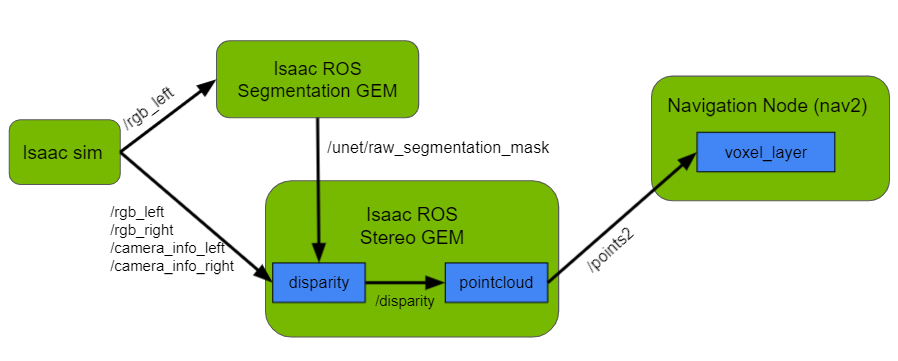
Figure 3 shows the fundamental workflow of the project.
You use a warehouse environment in NVIDIA Isaac Sim, which includes the Carter robot and forklifts. Following the ROS2 Navigation example, generate an occupancy map that is used by the Nav2 stack to avoid static obstacles like shelves. Dynamic or moving obstacles including forklifts and trolleys are added to the environment after creating the occupancy map. This is to mimic the real world, where objects change in the environment without the robot’s knowledge.
It is important to note the offset between the Carter robot’s left and right stereo cameras in NVIDIA Isaac Sim for the NVIDIA Isaac ROS Stereo GEM to generate disparity correctly. Ensure that the ROS2 bridge is enabled in NVIDIA Isaac Sim before starting simulation so that ROS2 messages can be communicated outside NVIDIA Isaac Sim.
NVIDIA Isaac ROS stereo GEM and Nav2
The Nav2 stack uses global and local costmaps to steer the robot clear of obstacles. The local costmap is updated based on new, moving obstacles in the environment and can take laser scans and point clouds as input from robotic sensors.
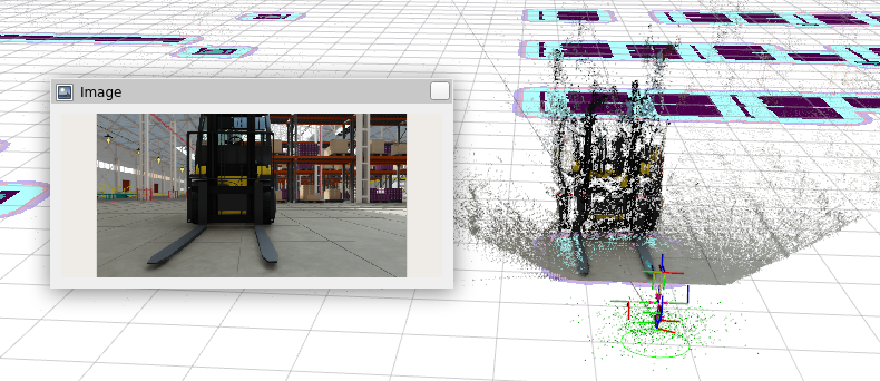
As laserscan from lidar fails to pick up forklift tines in real scenarios, you can address this problem by using point clouds from stereo images, which are passed to Nav2. These point clouds are generated using the NVIDIA Isaac ROS Stereo GEM.
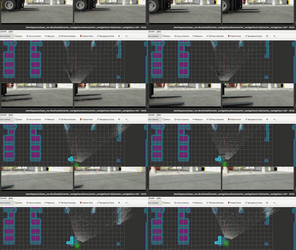
Figure 4. Point cloud generated using the NVIDIA Isaac ROS stereo GEM when the robot is in front of the forklift
On the right side of Figure 4, the light blue region under the tines shows that the Nav2 local costmap has been updated to represent an obstacle there, which the robot can now avoid. The average rate of images from NVIDIA Isaac Sim is 20 FPS and that of the point cloud from the stereo GEM is 16 FPS.
The stereo GEM generates a disparity image and then a point cloud for all objects that are seen in the left and right images from the robot’s cameras. Using the Isaac ROS segmentation GEM, this disparity can be filtered to generate a point cloud that includes only points belonging to objects of interest, for instance, forklift tines.
The next section explains this filtering in more detail.
Disparity filtering using the NVIDIA Isaac ROS segmentation GEM
Here’s how deep learning models trained on synthetically generated data can be used with NVIDIA Isaac ROS inference GEMs. You achieve the same goal: Help robots avoid forklift tines in simulation using the GEMs along with the Nav2 stack.
However, instead of generating a point cloud for all objects in the robot’s cameras’ field of view, you filter and generate a focused point cloud only for forklift tines.
Figure 5. Workflow to perform disparity filtering using NVIDIA Isaac ROS segmentation and stereo GEMs
I used a segmentation model trained on images of forklift tines. The NVIDIA Isaac ROS segmentation GEM takes RGB images from the robot in simulation and generates the corresponding segmentation images using the given model.
Any model can be used with this pipeline to filter specific objects based on the use case. Just generate (Replicator Composer) and train (TAO) on your data of interest!
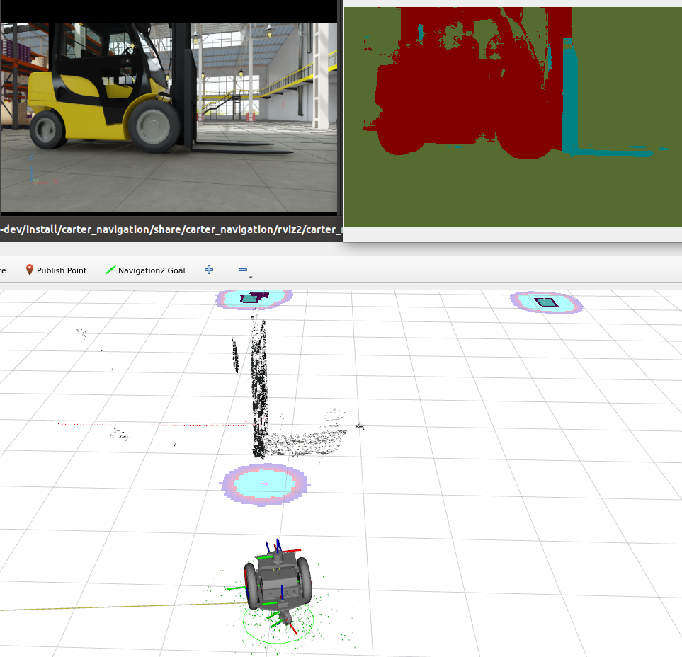
Figure 6. Colored segmentation image generated at 39 FPS by the trained model on images from the robot’s cameras. (top left) The robot’s left camera view. (top right) the segmentation mask; (bottom) the filtered point cloud for forklift tines.
Each pixel in the raw segmentation image represents the class label for the object at that location in the image. Knowing the label of interest, for instance, if 2 represents forklift tines, set the non-interest points to invalid in the corresponding disparity image generated by the Stereo GEM. The point cloud generated as a result does not include these points. This is helpful to reduce noise in the point cloud.
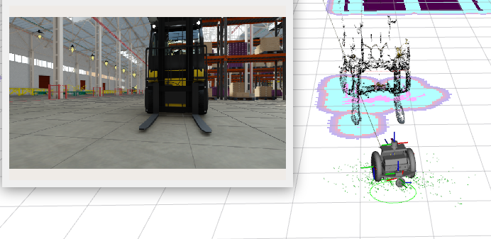
Figure 7. Point cloud generated after disparity filtering
Unlike the point cloud in Figure 4, this only has points belonging to forklift tines.
ROS domain IDs
As the NVIDIA Isaac ROS GEMs run within a container and NVIDIA Isaac Sim runs on the host, you must make sure that ROS topics can be communicated between the host and container.
For this, set the ROS domain ID of all processes to the same number. All ROS2 nodes using the same domain ID can communicate; those using different domain IDs cannot. For more information, see The ROS_DOMAIN_ID.
Notes
The workflow explained in this project avoids obstacles that can be detected by lidar and cameras. For obstacles that are too small or occluded, explore other sensors.
The approach is sensitive to disparity calculation and the quality of point cloud produced as a result. As calculating disparity is a challenging task, it is possible to get noisy point clouds that cause Nav2 to update the costmap incorrectly.
Disparity filtering is dependent on the performance of the segmentation model. A model that cannot produce accurate segmentation masks results in poorly filtered disparity and point clouds.
Here’s how to build efficient multi-camera pipelines taking advantage of the hardware accelerators on NVIDIA Jetson platform in just a few lines of Python.
Multi-camera applications are becoming increasingly popular; they are essential for enabling autonomous robots, intelligent video analytics (IVA), and AR/VR applications. Regardless of the specific use case, there are common tasks that must always be implemented:
Capture
Preprocessing
Encoding
Display
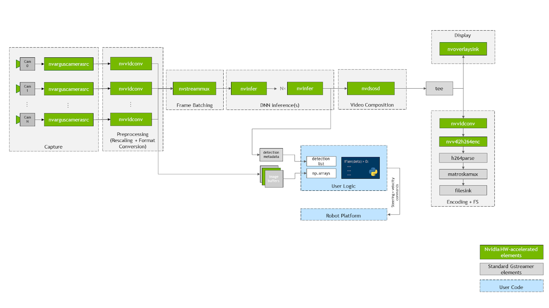
In many cases, you also want to deploy a DNN on the camera streams and run custom logic on the detections. Figure 1 shows the general flow of the application.
Figure 1. Flow of the pipeline implemented in this project
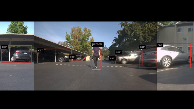
In this post, I showcase how to realize these common tasks efficiently on NVIDIA Jetson platform. Specifically, I present jetmulticam, an easy-to-use Python package for creating multi-camera pipelines. I demonstrate a specific use case on a robot with a surround camera system. Finally, I add custom logic (person following) based on the DNN object detections to obtain the results shown in the following video:
Video 1. Demo showing 3 independent cameras with ~270° field of view. Red Boxes correspond to DashCamNet detections, green ones to PeopleNet. The PeopleNet detections are used to perform person-following logic.
Multi-camera hardware
There are many parameters to consider when choosing a camera: resolution, frame rate, optics, global/rolling shutter, interface, pixel size, and so on. For more information about compatible cameras from NVIDIA partners, see the comprehensive list.
In this specific multi-camera setup, you use the following hardware:
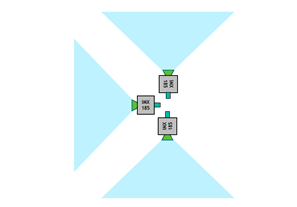
The IMX185 cameras each have a field of view of approximately 90°. Mount them orthogonally to one another for a total FOV of 270°, as shown in Figure 2.
Figure 2. Cameras are mounted to maximize the horizontal FOV
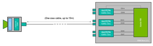
The cameras use the GMSL interface, which offers a lot of flexibility in positioning the cameras even meters away from the Jetson module. In this case, you can raise the cameras by ~0.5m to achieve a greater vertical FOV.
Figure 3. The GMSL interface enables the flexibility to position cameras away from the Jetson module
Getting started with Jetmulticam
First, download and install the NVIDIA Jetpack SDK on your Jetson board. Then, install the jetmulticam package:
After the setup, you can create a basic pipeline using the CameraPipeline class. Pass a list of cameras to include in the pipeline with the initializer argument. In the following example, the elements [0, 1, 2] correspond to device nodes /dev/video0, /dev/video1, and /dev/video2.
from jetmulticam import CameraPipeline
p = CameraPipeline([0, 1, 2])
And that’s it—the pipeline has been initialized and started. You can now read images from each camera in the pipeline and access them as numpy arrays.
img0 = p.read(0) # img0 is a np.array
img1 = p.read(1)
img2 = p.read(2)
Often, it is convenient to read from the camera in a loop, as in the following code example. The pipeline runs asynchronously from the main thread and read always gets the most recent buffer.
Now you can build a more complex pipeline. This time, use the CameraPipelineDNN class to compose a more complex pipeline, as well as two pretrained models from the NGC catalog: PeopleNet and DashCamNet.
import time from jetmulticam import CameraPipelineDNN from jetmulticam.models import PeopleNet, DashCamNet
while pipeline.running():
    arr = pipeline.images[0] # np.array with shape (1080, 1920, 3)
    dets = pipeline.detections[0] # Detections from the DNNs
    time.sleep(1/30)
Here’s the breakdown of the pipeline initialization:
Cameras
Models
Hardware acceleration
Saving video
Displaying video
Main loop
Cameras
Firstly, similarly to the previous example, the cameras argument is a list of sensors. In this case, you use cameras associated with device nodes:
/dev/video2
/dev/video5
/dev/video8
cameras=[2, 5, 8]
Models
The second argument, models, enables you to define pretrained models to run in the pipeline.
The models run in real time using NVIDIA Deep Learning Accelerator (DLA). Specifically, you deploy PeopleNet on DLA0 (DLA Core 0) and DashCamNet on DLA1.
Distributing models between two accelerators helps increase the total throughput of the pipeline. Furthermore, DLA is even more power-efficient than GPU. As a result, the system consumes as little as ~10W under full load with the highest clock settings. Finally, in this configuration, the Jetson GPU remains free to accelerate more tasks with the 384 CUDA cores available on Jetson NX.
The following code example shows the list of currently supported model/accelerator combinations.
As a final initialization step, configure the pipeline to display the video output on the screen for debugging purposes.
display=True
Main loop
Lastly, define the main loop. During runtime, the images are available under pipeline.images, and detection results under pipeline.detections.
while pipeline.running(): arr = pipeline.images[0] # np.array with shape (1080, 1920, 3) dets = pipeline.detections[0] # Detections from the DNNs time.sleep(1/30)
The following code example shows the resulting detections. For each detection, you get a dictionary containing the following:
Object class
Object position defined as [left, width, top, height] in pixel coordinates
As the last step, you can extend the main loop to build custom logic using the DNN output. Specifically, you use the detection outputs from your cameras to implement basic person-following logic in the robot. The source code is available in the NVIDIA-AI-IOT/jetson-multicamera-pipelines GitHub repo.
To find the human to follow, parse the pipeline.detections output. This logic is implemented in the find_closest_human function.
Calculate the robot’s steering angle based on where the bounding box is located in dets2steer.
If the human is in the left image, turn maximally left.
If the human is in right image, turn maximally right.
If the human is in the center image, turn proportionately to the X coordinate of the center of the bounding box.
The resulting video is saved to /home/nx/logs/videos, as you defined it during initialization.
Solution overview
Here’s a brief look at how jetmulticam works. The package dynamically creates and launches a GStreamer pipeline with the number of cameras that your application requires. Figure 4 shows how the underlying GStreamer pipeline looks when configured as in the person-following example. As you can see, all critical operations in the system, represented by green boxes, benefit from hardware acceleration.
Figure 4. Internal components of the jetmulticam package
First, the video is captured using multiple CSI cameras, using nvarguscamerasrc elements on the diagram. Each individual buffer is rescaled and converted to RGBA format with either nvvidconv or nvvideoconvert. Next, the frames are batched using the component provided by the DeepStream SDK. By default, the batch size is equal to the number of cameras in the system.
To deploy the DNN models, take advantage of the nvinfer elements. In the demo, I deployed two models, PeopleNet and DashCamNet, on two different accelerators, DLA core 1 and DLA core 2, both available on the Jetson Xavier NX. However, it is possible to stack even more models on top of each other, if needed.
After the resulting bounding boxes are overlaid by the nvosd element, you then display them on an HDMI display, using nvoverlaysink, as well as encoding the video stream with the hardware-accelerated H264 encoder. Save to a .mkv file.
The images available in the Python code (for example, pipeline.images[0]) are parsed to numpy arrays by a callback function, or probe, registered on each of the video converter elements. Similarly, another callback function is registered on the sinkpad of the last nvinfer element that parses the metadata into a user-friendly list of detections. For more information about the source code or individual component configuration, see the create_pipeline function.
Conclusion
The hardware acceleration available on the NVIDIA Jetson platform combined with NVIDIA SDKs enables you to achieve outstanding real-time performance. For example, the person-following example runs two object-detection neural networks in real time on three camera streams, all while maintaining CPU utilization under 20%.
The Jetmulticam package, showcased in this post, enables you to build your own hardware-accelerated pipelines in Python, and to include custom logic on top of the detections.
Read on step by step guide how hierarchical risk parity can used used in portfolio optimization to manage risk.
Data scientists often use the finance world as a playground for testing new techniques. Financial data has been recorded for decades, and it all takes on a numerical form, making it easy to process. Plus, there is always the chance that you create a model that makes money!
Within finance, the general goal of an investment is to maximize return (money made or lost on investment) while minimizing risk (the chance that the actual outcome differs from the predicted outcome). In short, investing money is all about the math.
This post introduces a portfolio optimization strategy that can help minimize exposure to risk. With access to a GPU, the algorithm can be sped-up by a factor up to 66x.
For retail investors, this speedup can be especially useful for frequent rebalances. Meanwhile, institutional investors can use this algorithm to manage money through a robo-advisor. Recalculating the algorithm for each unique customer’s portfolio can be computationally expensive, which can be greatly reduced by introducing a GPU.
In this post, I walk through a step-by-step guide introducing ML techniques for efficient portfolio allocation using hierarchical risk parity (HRP). This example uses Python with RAPIDS.
Choosing an algorithm for efficient financial predictions
In 1952, Harry Markowitz introduced a portfolio-optimization model known as the Modern Portfolio Theory. This model can generate a portfolio of investments that maximizes return for some given amount of risk.
Figure 1. Markowitz’s efficient frontier. Every portfolio lies in the blue area and aims to lie on the efficient frontier.
Unfortunately, the story does not end here. Markowitz’s Modern Portfolio Theory can only produce the most efficient portfolio if you know the risk and return of every equity to pick from. However, this does not always happen, because past performance is not indicative of future results.
For example, Verizon stock is highly correlated with AT&T. Therefore, Verizon competes for representation only against stocks like AT&T instead of against all equities in every sector.
Step-by-step guide to portfolio allocation with HRP
For the rest of this post, I focused on implementing HRP on RAPIDS and then comparing its performance to other common techniques.
Acquire data
In this post, I used daily adjusted close data from every security in the NASDAQ and NYSE over the period November 2018 to November 2021. This dataset was obtained through scripts from the NVIDIA/fsi-samples GitHub repo
For hardware, I used an i7 CPU with an NVIDIA Quadro 8000 GPU. For software, I used Python 3.9 with RAPIDS 22.02.
Wrangle data
Begin by reading in the datasets and aggregating them into a dataframe called m. Drop any equities with null values.
import cudf
m1 = cudf.read_csv("MVO3.2021.11/NASDAQ/prices.csv")
m2 = cudf.read_csv("MVO3.2021.11/NYSE/prices.csv")
m = cudf.concat([m1, m2], axis = 1)
m = m.dropna(axis = 1)
Some of the securities behave poorly: some stay flat for years, others contain non-positive values. Remove these bad securities.
data = m.values  # data.shape = (days, nAssets)
days = data.shape[0]
logRetAll = cp.log(data[1:, :]/data[:-1, :])
moveMask = cp.count_nonzero(logRetAll, axis = 0) > (days * 0.9)  # Require that each security moves day to day at least 90% of the time
positiveMask = data.min(axis = 0) > 0  # Require that all the data is positive
mask = moveMask & positiveMask
data = data[:, mask]
logRetAll = logRetAll[:, mask]
Next, split m into two parts: a training and testing period. The training period is from November 2018 to November 2020, while the testing occurs from November 2020 to November 2021.
As a result, you obtain the correlation and covariance matrices using built-in cuDF methods after creating a log returns matrix for the training data, as opposed to time series data.
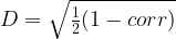
To cluster equities together, define a metric that gives the distance between two equities:
As correlation has a range of [-1, 1], you see that has the range [0, 1] where implies that and are perfectly correlated, and if , then and are perfectly uncorrelated.
Now that you can calculate the distance between two equities, cluster them so that like equities are clustered together.
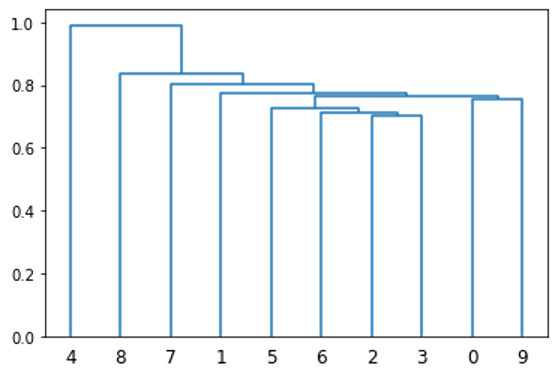
Each item is placed in its own cluster, and the two closest clusters are joined together. Then, recalculate the distance between this new cluster and all other clusters. Again, you combine the two closest clusters together. This process is repeated until there is only one cluster. One way to visualize this clustering is with a dendrogram.
from scipy.cluster.hierarchy import linkage, dendrogram
dendrogram(linkage(D[:10, :10].get()));
Figure 2. Dendrogram of the clustering of the first ten securities in D. The clustering algorithm is agglomerative clustering, or bottom-up clustering.
cuML has a built-in method to perform this function, which is used in the following code example. This is much faster than the linkage function from scipy, which performs similar functionality.
from cuml import AgglomerativeClustering as AC
# Create single linkage cluster using the Euclidean metric
def cluster(D):
    model=AC(affinity='l2', connectivity='pairwise', linkage='single')
    model.fit(D);
    return model.children_
cluster() outputs a 2 x N matrix where N is the number of equities in . The indices [0, i] and [1, i] represent the indices of the clusters joined for the i-th iteration.
Use matrix seriation
Next, produce an ordering from this clustering, which places like securities near each other. For example, the x-axis of Figure 2 provides an ordering of the first 10 stocks based on their clustering. This is done using an iterative implementation of matrix seriation, which is a common technique frequently used in archaeology.
def seriation(Z):
N = Z.shape[1]
stack = [2*N-2]
res_order = []
while(len(stack) != 0):
cur_idx = stack.pop()
if cur_idx
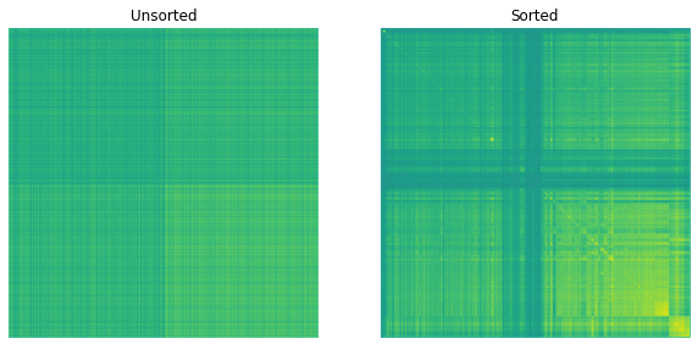
Figure 3 shows the resulting correlation matrices.
Figure 3. Heatmaps showing the correlation matrices before and after applying matrix seriation.
In Figure 3, you can observe patterns that emerge within the matrix when you apply your ordering to the correlation matrix. This indicates that similar equities are close to each other.
Assign weights
Finally, assign weights to the stocks. This is done through a recursive algorithm.
Split the sorted covariance matrix in half, calculating an adjusted amount of risk for each half, and then assigning weights to each half based on inverse variance portfolio (IVP) methodology. These steps are then repeated for each half.
IVP results in weights that are inversely proportional to the amount of risk, or variance, of the stock. That is, a high risk stock has low representation while a low risk stock has high representation.
Both HRP and IVP are risk-parity algorithms: they only take risk into account based on past performance.
def recursiveBisection(V, l, r, W):
#Performs recursive bisection weighting for a new portfolio
#V is the sorted correlation matrix
#l is the left index of the recursion
#r is the right index of the recursion
#W is the list of weights
if r-l == 1: #One item
return W
else:
#Split up V matrix
mid = l+(r-l)//2
V1 = V[l:mid, l:mid]
V2 = V[mid:r, mid:r]
#Find new adjusted V
V1_diag_inv = 1/cp.diag(V1)
V2_diag_inv = 1/cp.diag(V2)
w1 = V1_diag_inv/V1_diag_inv.sum()
w2 = V2_diag_inv/V2_diag_inv.sum()
V1_adj = w1.T@V1@w1
V2_adj = w2.T@V2@w2
#Adjust weights
a2 = V1_adj/(V1_adj+V2_adj)
a1 = 1-a2
W[l:mid] = W[l:mid]*a1
W[mid:r] = W[mid:r]*a2
W = recursiveBisection(V, l, mid, W)
W = recursiveBisection(V, mid, r, W)
return W
Analyze weights
You now have all of the tools necessary to perform HRP. See how it performs!
#Obtain the final weights and plot them
N = len(res_order)
V = covTrain[res_order, :][:, res_order]
W_tmp = recursiveBisection(V, 0, N, cp.ones(N))
W = cp.empty(len(W_tmp))
W[res_order] = W_tmp
plt.plot(W.get())
plt.xlabel("Security Index")
plt.ylabel("% allocation")
plt.title("HRP Allocation")
plt.plot();
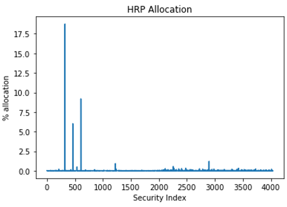
After applying the listed methods, you end up with a variable W that represents the weighting of each security.
Figure 4 displays the results.
Figure 4. Percent allocation for each security according to HRP methodology
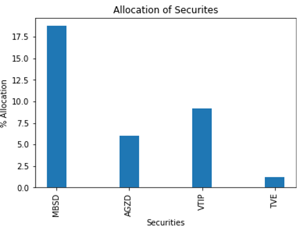
This graph is difficult to read. You can truncate it so that only securities with a weight greater than 1% are shown (Figure 5).
Figure 5. HRP final weights for securities that have a greater than 1% representation
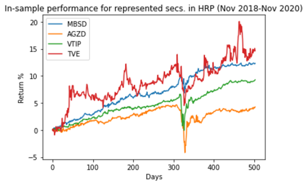
As a sanity check, Figure 6 shows how the top picks performed over the training period. You are looking to make sure that the securities have a relatively low volatility.
Figure 6. Performance of top HRP stocks during training period (Nov 2018 – Nov 2020)
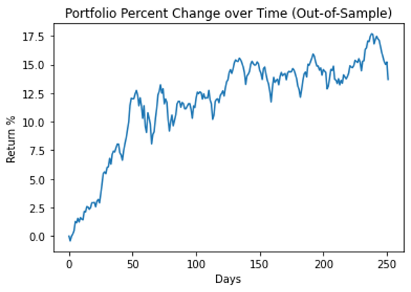
Figure 7 displays the performance of the entire portfolio over the testing period.
Figure 7. Performance of the HRP portfolio during the testing period (Nov 2020 – Nov 2021)
Compare against other portfolios
You can compare this performance to that of Modern Portfolio Theory. For this iteration, I chose to maximize the Sharpe ratio: a metric to track the performance of a portfolio.
In this formula, is the risk-free rate of return. In the finance world, risk is defined as where is the covariance matrix. This way, both the risk and return of a portfolio are folded into the metric.
Use scipy to perform numerical optimization.
from scipy.optimize import *
from scipy.optimize import *
def MPT(cov, R):
cons = [{'type': 'eq', 'fun': lambda x: sum(x) - 1}, #sum(w)==1",
{'type': 'ineq', 'fun': lambda x: x}] #each weight >=0 (no short selling)"
res = minimize(lambda x: -(x@R-1.025)/sqrt(x.T@cov@x), x0=np.ones(len(R))/len(R), constraints=cons) #Minimize risk"
return res.x
This is a complex numerical optimization problem, especially considering that you have over 4,000 assets. Shrink this to 278 securities by requiring that each must have a Sharpe ratio greater than 1. This cutoff is arbitrary, but masking is recommended to reduce runtime.
W_MPT = cp.zeros(nAssets)
sharpeTrain = (trainRetAll - 1.025) / (cp.std(logRetTrain, axis = 0) * math.sqrt(252)) # Annualized sharpe
covnp = covTrain[sharpeTrain > 1, :][:, sharpeTrain > 1].get() # Numpy version of covariance matrix over training period, masked
Rnp = trainRetAll[sharpeTrain > 1].get() # Return of all stocks over the training period, masked, in numpy
W_MPT[sharpeTrain > 1] = MPT(covnp, Rnp, 1+i/100)
You can also generate weights for the inverse variance portfolio.
Lastly, generate some random portfolios, which choose 15 different securities, and allocate a random amount to each one. This simulates a portfolio that an uninformed retail investor might choose.
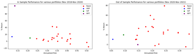
Figure 8 shows the outcomes of all portfolios.
Figure 8. Return vs. risk for the different portfolios over the training (left) and testing period (right)
For the preceding portfolios, you generate the Sharpe ratios in the following table.
Train (Nov 2018 – Nov 2020)
Test (Nov 2020 – Nov 2021)
Median of Random Portfolios
0.01
0.97
HRP
0.91
1.51
IVP
0.35
1.83
MPT
7.51
-0.18
Table 1. Sharpe ratios for four different portfolios over the training (left) and testing (right) period
While MPT has a high Sharpe ratio during the training sample, it turns negative during the training period, implying that the portfolio underperforms the risk-free rate of 2.5%. This demonstrates what is known as Markowitz’s curse: While it performs optimally in-sample, it oftentimes falls flat out-of-sample.
Further, while IVP has a higher Sharpe ratio than MPT over the testing period, remember that both of these methodologies are risk-parity portfolios. They aim to minimize risk and do not take return into account. It may be more pertinent to notice that over the testing period HRP has a 5.5% risk, while IVP has a 9.4% risk.
Analyze speed
One other thing to analyze is the runtime compared to a CPU. You can re-create the algorithm by using libraries such as SciPy, pandas, or NumPy instead of RAPIDS.
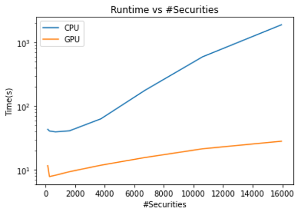
As the number of securities that you analyze increases, the amount of computing power required increases. This also increases the capability for parallelization, which can be captured by a GPU.
Figure 10. Log time vs. the number of securities for performing HRP on a GPU and CPU. The algorithm was run on mutual funds to give a larger pool of securities to run HRP on.
For the maximum number of securities, you achieve a speedup of 66x by running on a GPU over a CPU! Even in the worst case, you still obtain a 4x speedup.
Key learnings on HRP
Even though HRP was initially created to demonstrate how machine learning can be used in portfolio optimization, it has been shown to result possibly in less risk when compared to inverse variance and a higher Sharpe ratio than modern portfolio theory. López de Prado further backs this up in his Building Diversified Portfolios that Outperform Out of Sample paper, demonstrating lower drawdowns and variance for synthetic data.
Investors may turn to HRP when looking for ways to manage risk or to combine with other financial techniques to reduce risk for some requested rate of return.
With help from the GPU speedup that RAPIDS provides, HRP can be a viable portfolio optimization tool for a comparatively low computation cost.


 DataBloom
 Is there an ideal network design that always works? Let’s find out. This blog covers the pros and cons of pure layer 3, layer 2 only, and VXLAN and EVPN.
 To scale AI for financial services, companies must face several resource hurdles. The full-stack solution from NVIDIA and VMware helps you leverage the competitive advantages of AI.
 3D Artist Daniel Martinger discusses how he captured the attention of the computer graphics world with a path-traced rendered scene using an NVIDIA RTX 3090 and Unreal Engine 5.

![[Discussion] Training performance evaluation of MindSpore, a home-grown deep learning framework -- by ADSL Lab, CSU](https://b.thumbs.redditmedia.com/rTgUoc6iY7bYkQwi68EA3HYlQ8tdH4QRf0Rp7H-Eedk.jpg "[Discussion] Training performance evaluation of MindSpore, a home-grown deep learning framework -- by ADSL Lab, CSU")
 I show how NVIDIA Isaac Sim and NVIDIA Isaac ROS GEMs can be used with the Nav2 navigation stack for robotic navigation.
 Here’s how to build efficient multi-camera pipelines taking advantage of the hardware accelerators on NVIDIA Jetson platform in just a few lines of Python.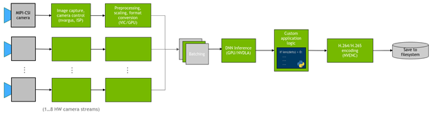
 Read on step by step guide how hierarchical risk parity can used used in portfolio optimization to manage risk.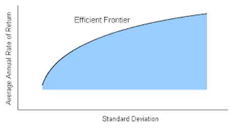



 is the risk-free rate of return. In the finance world, risk is defined as
  where
where  is the covariance matrix. This way, both the risk and return of a portfolio are folded into the metric.