Category: Misc

With the launch of Unreal Engine 5, NVIDIA announces support with key RTX technologies for developers to propel their games and experiences to the next level.

Unreal Engine is an open and advanced real-time 3D creation platform. Evolving from its state-of-the-art use in game engines into a multitude of industries, creators can deliver cutting-edge content, interactive experiences, and immersive virtual worlds. NVIDIA strives to simplify adoption of our technologies for developers to get hands on with leading-edge RTX technologies.

NVIDIA is supporting the launch of Unreal Engine 5 with key RTX technologies.Tens of thousands of developers leverage NVIDIA technologies and Unreal Engine to propel their games and experiences to the next level. You can get started building applications today.

We’ve created a series of introductory videos for NVIDIA technologies in UE5 including:

• Deep Learning Super Sampling (DLSS) 
• RTX Global Illumination (RTXGI)
• NVIDIA Reflex
• NVIDIA Omniverse Connector for UE5

The video below provides an overview for implementing ray tracing in Unreal Engine 5.

Deep Learning Super Sampling 

NVIDIA Deep Learning Super Sampling (DLSS) is a plug-in that uses deep learning algorithms to upscale or “super sample” an image, and helps during GPU heavy workloads like ray tracing. NVIDIA DLSS takes a lower resolution image and increases its resolution. 

Core benefits include uncompromised quality with higher performance. DLSS uses advanced AI rendering to produce image quality comparable to native resolution, and in some cases even better quality, while only conventionally rendering a fraction of the pixels. A new temporal feedback technique gives incredibly sharp image details and improved stability from frame to frame.

With DLSS, developers can choose among several image quality modes from Quality to Ultra Performance. Balancing quality and performance is done by controlling the game’s internal rendering resolution.

Additional benefits include:

•  NVIDIA Image Sharpening with a spatial upscaler and sharpening algorithm for non-RTX GPUs for cross-platform support.
• Deep Learning Anti-Aliasing mode or DLAA. This AI based anti-aliasing mode is for users with spare GPU headroom and looking for higher levels of image quality.

Get started with DLSS

To get started head to the DLSS download page, scroll down to the “Download UE Plugin” section, accept the terms of agreement, and launch the UE5 download link. Then you’re all set!  

For a more visual walkthrough on how to install and implement DLSS view the video below.

RTX Global Illumination

NVIDIA RTX Global Illumination (RTXGI) is a fast, high quality, and scalable real-time global illumination solution. It uses ray tracing to provide infinite bounce in indirect lighting, without the need to bake lighting or create multiple light setups for scenes. 

You can customize RTXGI to your needs on any DXR-enabled GPU, including the GeForce RTX 30 series, RTX 20 series, GTX 1660 series, and GTX 10 series. RTXGI’s scalable design gives you the control to decide when and where you want to crank up performance or max out image quality.

RTXGI is a plugin for UE5, however if you want more advanced features like indirect lighting in reflections and translucency support you can download the NVRTX branch.

Get started with RTXGI

To get started head to the download page and scroll down to the “Download UE Plugin” section, click the terms of agreement to start the UE5 download link, and you’re set.  

View how to install and implement RTXGI with the video below.

NVIDIA Reflex

The NVIDIA Reflex plug-in reduces system latency, which is key for any title where a responsive experience is required. With native support in Unreal Engine 5, simply navigate to the plug-ins folder in UE5, search for NVIDIA Reflex, and enable. 

Key features include:

• Low Latency Mode for reducing latency.
• Reflex Stats and Latency Markers. With Reflex Stats, gamers can get per-frame PC Latency without any special hardware. This metric is ideal for tweaking game, OS, and GPU settings. 
• Automatic Configuration and Flash Indicator for automatic configuration of the Reflex Analyzer. The Reflex Latency Analyzer detects clicks coming from your mouse and measures the time it takes for the resulting pixels (such as a gun muzzle flash) to change on screen. The results are displayed through GeForce Experience. 

Review the video walkthrough below for information on installing and implementing NVIDIA Reflex.

NVIDIA Omniverse Connector for Unreal Engine 5 preview

NVIDIA Omniverse is a 3D design collaboration and virtual world simulation platform for creators to connect and enhance 3D workflows. Developers can also easily build advanced 3D tools and expand their ecosystem reach.

At GTC 2022, NVIDIA introduced an updated Omniverse Connector for Unreal Engine including the ability to export the source geometry of Nanite meshes from Unreal Engine 5.

Review the Omniverse Connect documentation for information on installing and using Unreal Engine Omniverse Connector 104.1. For more information on Unreal Engine and NVIDIA technologies, visit our Unreal Engine developer page.

*Disclaimer:  All versions of these plug-ins have been tested on UE 5.0 Preview 2, and may not be compatible in the full release of Unreal Engine 5.0.

Pekka Varis’s artistry has come a long way from his early days as a self-styled “punk activist” who spray painted during the “old school days of hip hop in Finland.”

The post Meet the Omnivore: Videographer Makes Digital Walls, Virtual Homes Pop With NVIDIA Omniverse appeared first on NVIDIA Blog.

submitted by /u/the_Wallie
[visit reddit] [comments]

submitted by /u/kudoshinichi-8211
[visit reddit] [comments]

bert_output = BertLayer(n_fine_tune_layers=3, pooling="mean")(bert_inputs) bert_output = tf.keras.layers.Reshape((max_seq_length, embedding_size))(bert_output) bilstm = tf.keras.layers.Bidirectional(tf.keras.layers.LSTM(128, dropout=0.2,recurrent_dropout=0.2,return_sequences=True))(bert_output) output = tf.keras.layers.Dense(1, activation="softmax")(bilstm) model = tf.keras.models.Model(inputs=bert_inputs, outputs=output) model.compile(loss='binary_crossentropy', optimizer='adam', metrics=['accuracy']) model.summary() 

ValueError: A target array with shape (1288, 1) was passed for an output of shape (None, 256, 1) while using as loss `binary_crossentropy`. This loss expects targets to have the same shape as the output. 

submitted by /u/No-Life-8250
[visit reddit] [comments]

submitted by /u/Beginner_Journey
[visit reddit] [comments]

submitted by /u/shubham1300
[visit reddit] [comments]

The article includes a step by step explanation of the merge sort algorithm and code snippets illustrating the implementation of the algorithm itself.

Data Scientists deal with algorithms daily. However, the data science discipline as a whole has developed into a role that does not involve implementation of sophisticated algorithms. Nonetheless, practitioners can still benefit from building an understanding and repertoire of algorithms.

In this article, the sorting algorithm merge sort is introduced, explained, evaluated, and implemented. The aim of this post is to provide you with robust background information on the merge sort algorithm, which acts as foundational knowledge for more complicated algorithms.

Although merge sort is not considered to be complex, understanding this algorithm will help you recognize what factors to consider when choosing the most efficient algorithm to perform data-related tasks. Created in 1945, John Von Neumann developed the merge sort algorithm using the divide-and-conquer approach.

Divide and conquer

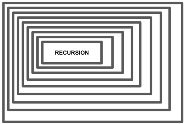
To understand the merge sort algorithm, you must be familiar with the divide and conquer paradigm, alongside the programming concept of recursion. Recursion within the computer science domain is when a method defined to solve a problem involves an invocation of itself within its implementation body.

In other words, the function calls itself repeatedly.

Divide and conquer algorithms (which merge sort is a type of) employ recursion within its approach to solve specific problems. Divide and conquer algorithms decompose complex problems into smaller sub-parts, where a defined solution is applied recursively to each sub-part. Each sub-part is then solved separately, and the solutions are recombined to solve the original problem.

The divide-and-conquer approach to algorithm design combines three primary elements:

• Decomposition of the larger problem into smaller subproblems. (Divide)
• Recursive utilization of functions to solve each of the smaller subproblems. (Conquer)
• The final solution is a composition of the solution to the smaller subproblems of the larger problem. (Combine)

Other algorithms use the divide-and-conquer paradigm, such as Quicksort, Binary Search, and Strassen’s algorithm.

Merge sort

In the context of sorting elements in a list and in ascending order, the merge sort method divides the list into halves, then iterates through the new halves, continually dividing them down further to their smaller parts.

Subsequently, a comparison of smaller halves is conducted, and the results are combined together to form the final sorted list.

Steps and implementation

Implementation of the merge sort algorithm is a three-step procedure. Divide, conquer, and combine.

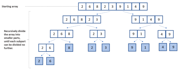
The divide component of the divide-and-conquer approach is the first step. This initial step separates the overall list into two smaller halves. Then, the lists are broken down further until they can no longer be divided, leaving only one element item in each halved list.

The recursive loop in merge sort’s second phase is concerned with the list’s elements being sorted in a particular order. For this scenario, the initial array is sorted in ascending order.

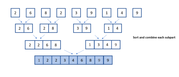
In the following illustration, you can see the division, comparison, and combination steps involved in the merge sort algorithm.

To implement this yourself:

• Create a function called merge_sort that accepts a list of integers as its argument. All following instructions presented are within this function.
• Start by dividing the list into halves. Record the initial length of the list.
• Check that the recorded length is equal to 1. If the condition evaluates to true, return the list as this means that there is just one element within the list. Therefore, there is no requirement to divide the list.
• Obtain the midpoint for a list with a number of elements greater than 1. When using the Python language, the // performs division with no remainder. It rounds the division result to the nearest whole number. This is also known as floor division.
• Using the midpoint as a reference point, split the list into two halves. This is the divide aspect of the divide-and-conquer algorithm paradigm.
• Recursion is leveraged at this step to facilitate the division of lists into halved components. The variables ‘left_half’ and ‘right_half’ are assigned to the invocation of the ‘merge_sort’ function, accepting the two halves of the initial list as parameters.
• The ‘merge_sort’ function returns the invocation of a function that merges two lists to return one combined, sorted list.

def merge_sort(list: [int]):
    list_length = len(list)
    
    if list_length == 1:
        return list
    
    mid_point = list_length // 2
    
    left_half = merge_sort(list[:mid_point])
    right_half = merge_sort(list[mid_point:])
    
    return merge(left_half, right_half)

• Create a ‘merge’ function that accepts two lists of integers as its arguments. This function contains the conquer and combine aspects of the divide-and-conquer algorithm paradigm. All following steps are executed within the body of this function.
• Assign an empty list to the variable ‘output’ that holds the sorted integers.
• The pointers ‘i’ and ‘j’ are used to index the left and right lists, respectively.
• Within the while loop, there is a comparison between the elements of both the left and right lists. After each comparison, the output list is populated within the two compared elements. The pointer of the list of the appended element is incremented.
• The remaining elements to be added to the sorted list are elements obtained from the current pointer value to the end of the respective list.

def merge(left, right):
    output = []
    i = j = 0
    
    while (i 

Performance and complexity

Big O notation is a standard for defining and organizing the performance of algorithms in terms of their space requirement and execution time.

Merge sort algorithm time complexity is the same for its best, worst, and average scenarios. For a list of size n, the expected number of steps, minimum number of steps, and maximum number of steps for the merge sort algorithm to complete, are all the same.

As noted earlier in this article, the merge sort algorithm is a three-step process: divide, conquer, and combine. The ‘divide’ step involves the computation of the midpoint of the list, which, regardless of the list size, takes a single operational step. Therefore the notation for this operation is denoted as O(1).

The ‘conquer’ step involves dividing and recursively solving subarrays–the notation log n denotes this. The ‘combine’ step consists of combining the results into a final list; this operation execution time is dependent on the list size and denoted as O(n).

The merge sort notation for its average, best, and worst time complexity is log n * n * O(1). In Big O notation, low-order terms and constants are negligible, meaning the final notation for the merge sort algorithm is O(n log n). For a detailed analysis of the merge sort algorithm, refer to this article.

Evaluation

Merge sort performs well when sorting large lists, but its operation time is slower than other sorting solutions when used on smaller lists. Another disadvantage of merge sort is that it will execute the operational steps even if the initial list is already sorted. In the use case of sorting linked lists, merge sort is one of the fastest sorting algorithms to use. Merge sort can be used in file sorting within external storage systems, such as hard drives.

Key takeaways

This article describes the merge sort technique by breaking it down in terms of its constituent operations and step-by-step processes.

Merge sort algorithm is commonly used and the intuition and implementation behind the algorithm is rather straightforward in comparison to other sorting algorithms. This article includes the implementation step of the merge sort algorithm in Python.

You should also know that the time complexity of the merge sort method’s execution time in different situations, remains the same for best, worst, and average scenarios. It is recommended that merge sort algorithm is applied in the following scenarios:

• When dealing with larger sets of data, use the merge sort algorithm. Merge sort performs poorly on small arrays when compared to other sorting algorithms.
• Elements within a linked list have a reference to the next element within the list. This means that within the merge sort algorithm operation, the pointers are modifiable, making the comparison and insertion of elements have a constant time and space complexity.
• Have some form of certainty that the array is unsorted. Merge sort will execute its operations even on sorted arrays, a waste of computing resources.
• Use merge sort when there is a consideration for the stability of data. Stable sorting involves maintaining the order of identical values within an array. When compared with the unsorted data input, the order of identical values throughout an array in a stable sort is kept in the same position in the sorted output.

submitted by /u/_padla_
[visit reddit] [comments]