Categories
Misc

Fetching AI Data: Researchers Get Leg Up on Teaching Dogs New Tricks with NVIDIA Jetson

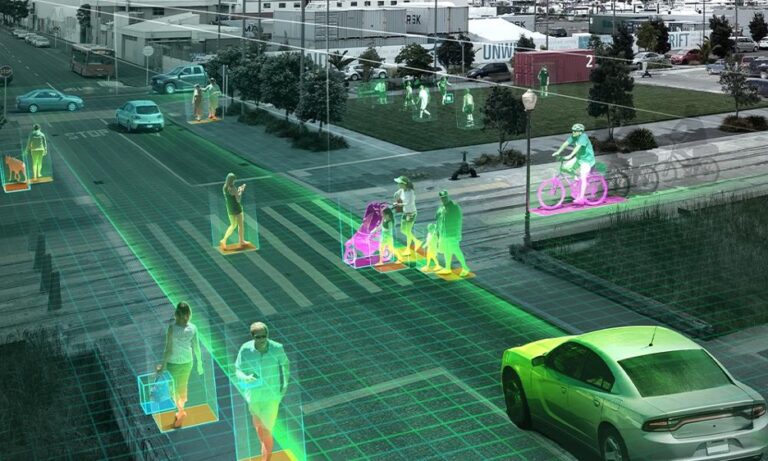
AI is going to the dogs. Literally. Colorado State University researchers Jason Stock and Tom Cavey have published a paper on an AI system to recognize and reward dogs for responding to commands. The graduate students in computer science trained image classification networks to determine whether a dog is sitting, standing or lying. If a Read article >

The post Fetching AI Data: Researchers Get Leg Up on Teaching Dogs New Tricks with NVIDIA Jetson appeared first on The Official NVIDIA Blog.

Categories
Misc

A Capital Calculator: Upstart Credits AI with Advancing Loans

With two early hits and the promise of more to come, it feels like a whole new ballgame in lending for Grant Schneider. The AI models he helped create as vice president of machine learning for Upstart are approving more personal loans at lower interest rates than the rules traditional banks use to gauge credit Read article >

The post A Capital Calculator: Upstart Credits AI with Advancing Loans appeared first on The Official NVIDIA Blog.

Categories
Misc

GFN Thursday Shines Ray-Traced Spotlight on Sweet Six-Pack of RTX Games

If Wednesday is hump day, GFN Thursday is the new official beginning of the weekend. We have a great lineup of games streaming from the cloud this week, with more details on that below. This GFN Thursday also spotlights some of the games using NVIDIA RTX tech, including a sweet six-pack that you’ll want to Read article >

The post GFN Thursday Shines Ray-Traced Spotlight on Sweet Six-Pack of RTX Games appeared first on The Official NVIDIA Blog.

Categories
Misc

torch, tidymodels, and high-energy physics

So what’s with the clickbait (high-energy physics)? Well, it’s not just clickbait. To showcase TabNet, we will be using the Higgs dataset (Baldi, Sadowski, and Whiteson (2014)), available at UCI Machine Learning Repository. I don’t know about you, but I always enjoy using datasets that motivate me to learn more about things. But first, let’s get acquainted with the main actors of this post!

TabNet

TabNet was introduced in Arik and Pfister (2020). It is interesting for three reasons:

  • It claims highly competitive performance on tabular data, an area where deep learning has not gained much of a reputation yet.

  • TabNet includes interpretability1 features by design.

  • It is claimed to significantly profit from self-supervised pre-training, again in an area where this is anything but undeserving of mention.

In this post, we won’t go into (3), but we do expand on (2), the ways TabNet allows access to its inner workings.

How do we use TabNet from R? The torch ecosystem includes a package – tabnet – that not only implements the model of the same name, but also allows you to make use of it as part of a tidymodels workflow.

tidymodels

To many R-using data scientists, the tidymodels framework will not be a stranger. tidymodels provides a high-level, unified approach to model training, hyperparameter optimization, and inference.

tabnet is the first (of many, we hope) torch models that let you use a tidymodels workflow all the way: from data pre-processing over hyperparameter tuning to performance evaluation and inference. While the first, as well as the last, may seem nice-to-have but not “mandatory”, the tuning experience is likely to be something you’ll won’t want to do without!

Using tabnet with tidymodels

In this post, we first showcase a tabnet-using workflow in a nutshell, making use of hyperparameter settings reported in the paper.

Then, we initiate a tidymodels-powered hyperparameter search, focusing on the basics but also, encouraging you to dig deeper at your leisure.

Finally, we circle back to the promise of interpretability, demonstrating what is offered by tabnet and ending in a short discussion.

In the flow with TabNet

As usual, we start by loading all required libraries. We also set a random seed, on the R as well as the torch sides. When model interpretation is part of your task, you will want to investigate the role of random initialization.

library(torch)
library(tabnet)
library(tidyverse)
library(tidymodels)
library(finetune) # to use tuning functions from the new finetune package
library(vip) # to plot feature importances

set.seed(777)
torch_manual_seed(777)

Next, we load the dataset.

# download from https://archive.ics.uci.edu/ml/datasets/HIGGS
higgs <- read_csv(
  "HIGGS.csv",
  col_names = c("class", "lepton_pT", "lepton_eta", "lepton_phi", "missing_energy_magnitude",
                "missing_energy_phi", "jet_1_pt", "jet_1_eta", "jet_1_phi", "jet_1_b_tag",
                "jet_2_pt", "jet_2_eta", "jet_2_phi", "jet_2_b_tag", "jet_3_pt", "jet_3_eta",
                "jet_3_phi", "jet_3_b_tag", "jet_4_pt", "jet_4_eta", "jet_4_phi", "jet_4_b_tag",
                "m_jj", "m_jjj", "m_lv", "m_jlv", "m_bb", "m_wbb", "m_wwbb"),
  col_types = "fdddddddddddddddddddddddddddd"
  )

What’s this about? In high-energy physics, the search for new particles takes place at powerful particle accelerators, such as (and most prominently) CERN’s Large Hadron Collider. In addition to actual experiments, simulation plays an important role. In simulations, “measurement” data are generated according to different underlying hypotheses, resulting in distributions that can be compared with each other. Given the likelihood of the simulated data, the goal then is to make inferences about the hypotheses.

The above dataset (Baldi, Sadowski, and Whiteson (2014)) results from just such a simulation. It explores what features could be measured assuming two different processes. In the first process, two gluons collide, and a heavy Higgs boson is produced; this is the signal process, the one we’re interested in. In the second, the collision of the gluons results in a pair of top quarks – this is the background process.

Through different intermediaries, both processes result in the same end products – so tracking these does not help. Instead, what the paper authors did was simulate kinematic features (momenta, specifically) of decay products, such as leptons (electrons and protons) and particle jets. In addition, they constructed a number of high-level features, features that presuppose domain knowledge. In their article, they showed that, in contrast to other machine learning methods, deep neural networks did nearly as well when presented with the low-level features (the momenta) only as with just the high-level features alone.

Certainly, it would be interesting to double-check these results on tabnet, and then, look at the respective feature importances. However, given the size of the dataset, non-negligible computing resources (and patience) will be required.

Speaking of size, let’s take a look:

higgs %>% glimpse()
Rows: 11,000,000
Columns: 29
$ class                    <fct> 1.000000000000000000e+00, 1.000000…
$ lepton_pT                <dbl> 0.8692932, 0.9075421, 0.7988347, 1…
$ lepton_eta               <dbl> -0.6350818, 0.3291473, 1.4706388, …
$ lepton_phi               <dbl> 0.225690261, 0.359411865, -1.63597…
$ missing_energy_magnitude <dbl> 0.3274701, 1.4979699, 0.4537732, 1…
$ missing_energy_phi       <dbl> -0.68999320, -0.31300953, 0.425629…
$ jet_1_pt                 <dbl> 0.7542022, 1.0955306, 1.1048746, 1…
$ jet_1_eta                <dbl> -0.24857314, -0.55752492, 1.282322…
$ jet_1_phi                <dbl> -1.09206390, -1.58822978, 1.381664…
$ jet_1_b_tag              <dbl> 0.000000, 2.173076, 0.000000, 0.00…
$ jet_2_pt                 <dbl> 1.3749921, 0.8125812, 0.8517372, 2…
$ jet_2_eta                <dbl> -0.6536742, -0.2136419, 1.5406590,…
$ jet_2_phi                <dbl> 0.9303491, 1.2710146, -0.8196895, …
$ jet_2_b_tag              <dbl> 1.107436, 2.214872, 2.214872, 2.21…
$ jet_3_pt                 <dbl> 1.1389043, 0.4999940, 0.9934899, 1…
$ jet_3_eta                <dbl> -1.578198314, -1.261431813, 0.3560…
$ jet_3_phi                <dbl> -1.04698539, 0.73215616, -0.208777…
$ jet_3_b_tag              <dbl> 0.000000, 0.000000, 2.548224, 0.00…
$ jet_4_pt                 <dbl> 0.6579295, 0.3987009, 1.2569546, 0…
$ jet_4_eta                <dbl> -0.01045457, -1.13893008, 1.128847…
$ jet_4_phi                <dbl> -0.0457671694, -0.0008191102, 0.90…
$ jet_4_btag               <dbl> 3.101961, 0.000000, 0.000000, 0.00…
$ m_jj                     <dbl> 1.3537600, 0.3022199, 0.9097533, 0…
$ m_jjj                    <dbl> 0.9795631, 0.8330482, 1.1083305, 1…
$ m_lv                     <dbl> 0.9780762, 0.9856997, 0.9856922, 0…
$ m_jlv                    <dbl> 0.9200048, 0.9780984, 0.9513313, 0…
$ m_bb                     <dbl> 0.7216575, 0.7797322, 0.8032515, 0…
$ m_wbb                    <dbl> 0.9887509, 0.9923558, 0.8659244, 1…
$ m_wwbb                   <dbl> 0.8766783, 0.7983426, 0.7801176, 0…

Eleven million “observations” (kind of) – that’s a lot! Like the authors of the TabNet paper (Arik and Pfister (2020)), we’ll use 500,000 of these for validation. (Unlike them, though, we won’t be able to train for 870,000 iterations!)

The first variable, class, is either 1 or 0, depending on whether a Higgs boson was present or not. While in experiments, only a tiny fraction of collisions produce one of those, both classes are about equally frequent in this dataset.

As for the predictors, the last seven are high-level (derived). All others are “measured”.

Data loaded, we’re ready to build a tidymodels workflow, resulting in a short sequence of concise steps.

First, split the data:

n <- 11000000
n_test <- 500000
test_frac <- n/n_all

split <- initial_time_split(higgs, prop = 1 - test_frac)
train <- training(split)
test  <- testing(split)

Second, create a recipe. We want to predict class from all other features present:

rec <- recipe(class ~ ., train) 

Third, create a parsnip model specification of class tabnet. The parameters passed are those reported by the TabNet paper, for the S-sized model variant used on this dataset.2

# hyperparameter settings (apart from epochs) as per the TabNet paper (TabNet-S)
mod <- tabnet(epochs = 3, batch_size = 16384, decision_width = 24, attention_width = 26,
              num_steps = 5, penalty = 0.000001, virtual_batch_size = 512, momentum = 0.6,
              feature_reusage = 1.5, learn_rate = 0.02) %>%
  set_engine("torch", verbose = TRUE) %>%
  set_mode("classification")

Fourth, bundle recipe and model specifications in a workflow:

wf <- workflow() %>%
  add_model(mod) %>%
  add_recipe(rec)

Fifth, train the model. This will take some time. Training finished, we save the trained parsnip model, so we can reuse it at a later time.

fitted_model <- wf %>% fit(train)

# access the underlying parsnip model and save it to RDS format
# depending on when you read this, a nice wrapper may exist
# see https://github.com/mlverse/tabnet/issues/27  
fitted_model$fit$fit$fit %>% saveRDS("saved_model.rds")

After three epochs, loss was at 0.609.

Sixth – and finally – we ask the model for test-set predictions and have accuracy computed.

preds <- test %>% 
  bind_cols(predict(fitted_model, test))

yardstick::accuracy(preds, class, .pred_class)
# A tibble: 1 x 3
  .metric  .estimator .estimate
  <chr>    <chr>          <dbl>
1 accuracy binary         0.672

We didn’t quite arrive at the accuracy reported in the TabNet paper (0.783), but then, we only trained for a tiny fraction of the time.

In case you’re thinking: well, that was a nice and effortless way of training a neural network! – just wait and see how easy hyperparameter tuning can get. In fact, no need to wait, we’ll take a look right now.

TabNet tuning

For hyperparameter tuning, the tidymodels framework makes use of cross-validation. With a dataset of considerable size, some time and patience is needed; for the purpose of this post, I’ll use 1/1,000 of observations.

Changes to the above workflow start at model specification. Let’s say we’ll leave most settings fixed, but vary the TabNet-specific hyperparameters decision_width, attention_width, and num_steps, as well as the learning rate:3

mod <- tabnet(epochs = 1, batch_size = 16384, decision_width = tune(), attention_width = tune(),
              num_steps = tune(), penalty = 0.000001, virtual_batch_size = 512, momentum = 0.6,
              feature_reusage = 1.5, learn_rate = tune()) %>%
  set_engine("torch", verbose = TRUE) %>%
  set_mode("classification")

Workflow creation looks the same as before:

wf <- workflow() %>%
  add_model(mod) %>%
  add_recipe(rec)

Next, we specify the hyperparameter ranges we’re interested in, and call one of the grid construction functions from the dials package to build one for us. If it wasn’t for demonstration purposes, we’d probably want to have more than eight alternatives though, and pass a higher size to grid_max_entropy() .

grid <-
  wf %>%
  parameters() %>%
  update(
    decision_width = decision_width(range = c(20, 40)),
    attention_width = attention_width(range = c(20, 40)),
    num_steps = num_steps(range = c(4, 6)),
    learn_rate = learn_rate(range = c(-2.5, -1))
  ) %>%
  grid_max_entropy(size = 8)

grid
# A tibble: 8 x 4
  learn_rate decision_width attention_width num_steps
       <dbl>          <int>           <int>     <int>
1    0.00529             28              25         5
2    0.0858              24              34         5
3    0.0230              38              36         4
4    0.0968              27              23         6
5    0.0825              26              30         4
6    0.0286              36              25         5
7    0.0230              31              37         5
8    0.00341             39              23         5

To search the space, we use tune_race_anova() from the new finetune package, making use of five-fold cross-validation:

ctrl <- control_race(verbose_elim = TRUE)
folds <- vfold_cv(train, v = 5)
set.seed(777)

res <- wf %>% 
    tune_race_anova(
    resamples = folds, 
    grid = grid,
    control = ctrl
  )

We can now extract the best hyperparameter combinations:

res %>% show_best("accuracy") %>% select(- c(.estimator, .config))
# A tibble: 5 x 8
  learn_rate decision_width attention_width num_steps .metric   mean     n std_err
       <dbl>          <int>           <int>     <int> <chr>    <dbl> <int>   <dbl>
1     0.0858             24              34         5 accuracy 0.516     5 0.00370
2     0.0230             38              36         4 accuracy 0.510     5 0.00786
3     0.0230             31              37         5 accuracy 0.510     5 0.00601
4     0.0286             36              25         5 accuracy 0.510     5 0.0136 
5     0.0968             27              23         6 accuracy 0.498     5 0.00835

It’s hard to imagine how tuning could be more convenient!

Now, we circle back to the original training workflow, and inspect TabNet’s interpretability features.

TabNet interpretability features

TabNet’s most prominent characteristic is the way – inspired by decision trees – it executes in distinct steps. At each step, it again looks at the original input features, and decides which of those to consider based on lessons learned in prior steps. Concretely, it uses an attention mechanism to learn sparse masks which are then applied to the features.

Now, these masks being “just” model weights means we can extract them and draw conclusions about feature importance. Depending on how we proceed, we can either

  • aggregate mask weights over steps, resulting in global per-feature importances;

  • run the model on a few test samples and aggregate over steps, resulting in observation-wise feature importances; or

  • run the model on a few test samples and extract individual weights observation- as well as step-wise.

This is how to accomplish the above with tabnet.

Per-feature importances

We continue with the fitted_model workflow object we ended up with at the end of part 1. vip::vip is able to display feature importances directly from the parsnip model:

fit <- pull_workflow_fit(fitted_model)
vip(fit) + theme_minimal()
Global feature importances.

(#fig:unnamed-chunk-16)Global feature importances.

Together, two high-level features dominate, accounting for nearly 50% of overall attention. Along with a third high-level feature, ranked in place four, they occupy about 60% of “importance space”.

Observation-level feature importances

We choose the first hundred observations in the test set to extract feature importances. Due to how TabNet enforces sparsity, we see that many features have not been made use of:

ex_fit <- tabnet_explain(fit$fit, test[1:100, ])

ex_fit$M_explain %>%
  mutate(observation = row_number()) %>%
  pivot_longer(-observation, names_to = "variable", values_to = "m_agg") %>%
  ggplot(aes(x = observation, y = variable, fill = m_agg)) +
  geom_tile() +
  theme_minimal() + 
  scale_fill_viridis_c()
Per-observation feature importances.

(#fig:unnamed-chunk-18)Per-observation feature importances.

Per-step, observation-level feature importances

Finally and on the same selection of observations, we again inspect the masks, but this time, per decision step:

ex_fit$masks %>% 
  imap_dfr(~mutate(
    .x, 
    step = sprintf("Step %d", .y),
    observation = row_number()
  )) %>% 
  pivot_longer(-c(observation, step), names_to = "variable", values_to = "m_agg") %>% 
  ggplot(aes(x = observation, y = variable, fill = m_agg)) +
  geom_tile() +
  theme_minimal() + 
  theme(axis.text = element_text(size = 5)) +
  scale_fill_viridis_c() +
  facet_wrap(~step)
Per-observation, per-step feature importances.

(#fig:unnamed-chunk-20)Per-observation, per-step feature importances.

This is nice: We clearly see how TabNet makes use of different features at different times.

So what do we make of this? It depends. Given the enormous societal importance of this topic – call it interpretability, explainability, or whatever – let’s finish this post with a short discussion.

Interpretable, explainable, …? Beyond the arbitrariness of definitions

An internet search for “interpretable vs. explainable ML” immediately turns up a number of sites confidently stating “interpretable ML is …” and “explainable ML is …”, as though there were no arbitrariness in common-speech definitions. Going deeper, you find articles such as Cynthia Rudin’s “Stop Explaining Black Box Machine Learning Models for High Stakes Decisions and Use Interpretable Models Instead” (Rudin (2018)) that present you with a clear-cut, deliberate, instrumentalizable distinction that can actually be used in real-world scenarios.

In a nutshell, what she decides to call explainability is: approximate a black-box model by a simpler (e.g., linear) model and, starting from the simple model, make inferences about how the black-box model works. One of the examples she gives for how this could fail is so striking I’d like to fully cite it:

Even an explanation model that performs almost identically to a black box model might use completely different features, and is thus not faithful to the computation of the black box. Consider a black box model for criminal recidivism prediction, where the goal is to predict whether someone will be arrested within a certain time after being released from jail/prison. Most recidivism prediction models depend explicitly on age and criminal history, but do not explicitly depend on race. Since criminal history and age are correlated with race in all of our datasets, a fairly accurate explanation model could construct a rule such as “This person is predicted to be arrested because they are black.” This might be an accurate explanation model since it correctly mimics the predictions of the original model, but it would not be faithful to what the original model computes.

What she calls interpretability, in contrast, is deeply related to domain knowledge:

Interpretability is a domain-specific notion […] Usually, however, an interpretable machine learning model is constrained in model form so that it is either useful to someone, or obeys structural knowledge of the domain, such as monotonicity [e.g.,8], causality, structural (generative) constraints, additivity [9], or physical constraints that come from domain knowledge. Often for structured data, sparsity is a useful measure of interpretability […]. Sparse models allow a view of how variables interact jointly rather than individually. […] e.g., in some domains, sparsity is useful,and in others is it not.

If we accept these well-thought-out definitions, what can we say about TabNet? Is looking at attention masks more like constructing a post-hoc model or more like having domain knowledge incorporated? I believe Rudin would argue the former, since

  • the image-classification example she uses to point out weaknesses of explainability techniques employs saliency maps, a technical device comparable, in some ontological sense, to attention masks;

  • the sparsity enforced by TabNet is a technical, not a domain-related constraint;

  • we only know what features were used by TabNet, not how it used them.

On the other hand, one could disagree with Rudin (and others) about the premises. Do explanations have to be modeled after human cognition to be considered valid? Personally, I guess I’m not sure, and to cite from a post by Keith O’Rourke on just this topic of interpretability,

As with any critically-thinking inquirer, the views behind these deliberations are always subject to rethinking and revision at any time.

In any case though, we can be sure that this topic’s importance will only grow with time. While in the very early days of the GDPR (the EU General Data Protection Regulation) it was said that Article 22 (on automated decision-making) would have significant impact on how ML is used4, unfortunately the current view seems to be that its wordings are far too vague to have immediate consequences (e.g., Wachter, Mittelstadt, and Floridi (2017)). But this will be a fascinating topic to follow, from a technical as well as a political point of view.

Thanks for reading!

Arik, Sercan O., and Tomas Pfister. 2020. “TabNet: Attentive Interpretable Tabular Learning.” http://arxiv.org/abs/1908.07442.

Baldi, P., P. Sadowski, and D. Whiteson. 2014. “Searching for exotic particles in high-energy physics with deep learning.” Nature Communications 5 (July): 4308. https://doi.org/10.1038/ncomms5308.

Rudin, Cynthia. 2018. “Stop Explaining Black Box Machine Learning Models for High Stakes Decisions and Use Interpretable Models Instead.” http://arxiv.org/abs/1811.10154.

Wachter, Sandra, Brent Mittelstadt, and Luciano Floridi. 2017. “Why a Right to Explanation of Automated Decision-Making Does Not Exist in the General Data Protection Regulation.” International Data Privacy Law 7 (2): 76–99. https://doi.org/10.1093/idpl/ipx005.

  1. I’m using the term “naively” here. For a short discussion, see the final section, [Interpretable, explainable, you tell me – beyond arbitrary definitions].↩︎

  2. Apart from the number of epochs, that is.↩︎

  3. The number of epochs is set to one for demonstration purposes only; in reality, you will want to tune this as well.↩︎

  4. See, e.g., <http://www.odbms.org/2018/07/ai-machine-learning-and-the-gdpr-are-the-wild-west-days-of-advanced-analytics-over/>.↩︎

Categories
Misc

Webinar: Top 11 Questions from “Ray Tracing with Unity’s High Definition Render Pipeline”

The recent webinar shares how to use Unity’s High Definition Render Pipeline (HDRP) wizard to enable ray-tracing in your Unity project with just a few clicks.

The recent webinar shares how to use Unity’s High Definition Render Pipeline (HDRP) wizard to enable ray-tracing in your Unity project with just a few clicks. At the end of the webinar, we hosted a Q&A session with our guest speakers from Unity Pierre Yves Donzallaz and Anis Benyoub and below are the top 11 questions asked.

Q: What are the specifications of the computer used for the webinar?

Pierre: The computer hosts an NVIDIA RTX 2070 Super, with a 16-thread CPU and 32 GB of system memory. It is a typical midrange configuration for a gaming machine nowadays. Performance is great when using ray traced shadows and ambient occlusion (60+ fps), or only ray-traced reflections in the Performance mode. Nevertheless, the frame rate may dip under 30 fps at 1080p when combining high quality ray traced global illumination, reflections, ambient occlusion, and shadows. This is naturally expected, especially when compared to other games using many ray tracing effects at once.

Q: Can ray tracing be used for very large open architectural scenes, where rays need to travel hundreds of meters?

Anis: Yes, Unity’s HDRP does not limit the length of the rays in its latest version. Therefore, you can tune the ray length of the effects you want to use, as well as increase the range of the Light Cluster, which is a structure listing the local lights and reflection probes active in each of its cells. 

Q: What are the minimum requirements to achieve good performance with ray tracing?

Pierre: It entirely depends on the number of ray tracing effects you want to enable and their quality (e.g. number of bounces and samples). For instance, for game scenarios with ray traced shadows and ray traced ambient occlusion only, an NVIDIA RTX 2060 Super could be an acceptable solution. However, it greatly depends on the optimization of the project itself. For high-end gaming, with all effects enabled, an RTX 2080 or better is highly recommended. Finally, for visualization and “interactive frame rate” scenarios, an RTX 3000 series or better will certainly offer the most comfortable working experience.

Q: Does the scene have to be pre-baked in any way to use ray tracing and/or path tracing?

Pierre: The path tracer does not require any pre-baking, thanks to its more brute force (and slower) approach to lighting. In some cases, ray tracing can take advantage of a better lighting baseline—one example is in the form of local reflection probes, notably in darker interiors where a fallback to the skybox’s reflection probe is unwanted. For a bright outdoor scene with a lot of sun and sky contribution, no baking at all is required to take advantage of the ray tracing, as the fallback to the ambient probe and reflection probe derived automatically from the sky will offer a good starting point.

Image courtesy of Unity Technologies

Q: Are single-sided objects problematic with ray tracing and/or path tracing,  for example, a floor or a ceiling plane?

Anis: Ray tracing and path tracing in Unity have the same visibility requirements as the rasterized techniques: proper shadow casting is expected, either in the form of a watertight mesh, a shadow proxy like in our new HDRP Scene Template, or in the form of double-sided materials or two-sided shadows. 

Q: Is it possible to tune the ray tracing settings on a per scene or per location basis? 

Pierre: Certainly. Unity’s HDRP uses a Volume system to control precisely settings applied spatially, depending on the camera position. The shape of a volume can be a box, a sphere, a custom mesh (concave), or it can be infinitely large (global). Multiple volumes can be nested, thanks to the priority system, and smooth transitions can be achieved easily by tweaking the blend distances or the influence of each volume. Of course with Unity, you can easily adjust the volume settings programmatically if needed.

Q: Do I have to use Temporal Anti Aliasing (TAA) to use ray tracing? 

Pierre: TAA can help dramatically, so it is highly recommended. However, it isn’t mandatory. The temporal accumulation helps reduce high-frequency noise whenever the denoiser is unable to provide good results due to a lack of history, typically with moving objects, such as trees moving in the wind.

Q: Does the image converge faster on more powerful hardware?

Anis: To obtain an image with a minimal amount of noise, the image requires a few frames to stabilize. Therefore, with a more powerful GPU and the resulting higher frame rate (uncapped), your frame time will be lowered and you will get a stable image more rapidly. 

Q: During the development of this demo, what was the most exciting feature you worked on or experienced?

Pierre: Personally, playing with mirrors and increasing the number of bounces for the ray-traced reflections beyond a handful was particularly impressive. Of course, the use cases for multi-bounce reflections are fairly limited in common projects, and two or three bounces will suffice in most real life-like cases. Nonetheless, it is always fun to watch recursive reflections!

Q: How much further can this technology go? It looks almost as close to real life as possible based on the examples shown in the webinar.

Anis: Real-time path tracing is certainly the goal in the distant future. However, it will require further research on real-time path tracing denoisers. In the meantime, a hybrid pipeline like the one offered by Unity’s HDRP, with a mix of rasterized and ray traced effects can already offer a great compromise on current hardware.

Q: Can we achieve “physically accurate” results in terms of lumen levels? For technical lighting analysis.

Pierre: Unity’s HDRP provides physical light units (lux, lumen, candela, EV, and nits) and physically based light attenuation. Therefore, results can be somewhat close to reality when using the GPU Lightmapper, the path tracer, or the ray traced global illumination with a sufficient number of samples. However, keep in mind that all these features are mere approximations of real-life physics and should be taken with a grain of salt. For technical lighting analysis, you will also certainly be interested in our improved exposure debug views, which offer an EV100 visualization of the scene for example.

Image courtesy of Unity Technologies

To learn more, visit the developer ray tracing resources page where you can find videos, blogs, webinars, and more to help you get started. 

And don’t miss out on the latest ray tracing news – GTC starts April 12, 2021, and registration is free. Be the first to know when registration is open. 

Categories
Misc

I want to add another step here where after reading the images the dataset is split into the image (X) and the BBox (Y) information as TensorFlow objects for RESNET50. Should I index through the ds_train or there is a better way. Thank you.

submitted by /u/dirtygrip
[visit reddit] [comments]

Categories
Misc

NVIDIA Releases Updates to CUDA-X AI Libraries

NVIDIA CUDA-X AI are deep learning libraries for researchers and software developers to build high performance GPU-accelerated applications for conversational AI, recommendation systems and computer vision.

NVIDIA CUDA-X AI are deep learning libraries for researchers and software developers to build high performance GPU-accelerated applications for conversational AI, recommendation systems and computer vision. CUDA-X AI libraries deliver world leading performance for both training and inference across industry benchmarks such as MLPerf.

Learn what’s new in the latest releases of CUDA-X AI libraries and NGC.

Refer to each package’s release notes in documentation for additional information.

cuDNN 8.1

The NVIDIA CUDA Deep Neural Network library (cuDNN) is a GPU-accelerated library of primitives for deep neural networks. This version of cuDNN includes:

TensorRT 7.2

NVIDIA TensorRT is a platform for high-performance deep learning inference. This version of TensorRT includes:

  • New debugging APIs – ONNX Graphsurgeon, Polygraphy, and Pytorch Quantization toolkit
  • Support for Python 3.8 

In addition this version includes several bug fixes and documentation upgrades.

Triton Inference Server 2.6

Triton is an open source inference serving software designed to maximize performance and simplify production deployment at scale. This version of Triton includes:

  • Alpha version of Windows build, which supports gRPC and TensorRT backend
  • Initial release of Model Analyzer, which is a tool that helps users select the optimal model configuration that maximizes performance in Triton.
  • Support for Ubuntu 20.04 – Triton provides support for the latest version of Ubuntu, which comes with additional security updates.
  • Native support in DeepStream – Triton on DeepStream can run inference on video analytics workflows on the edge or on the cloud with Kubernetes.

NGC Container Registry

NGC, the hub for GPU-optimized AI/ML/HPC application containers, models and SDKs that simplifies software development and deployment so users can achieve faster time to solution. This month’s updates include:

  • NGC catalog in the AWS Marketplace – users can now pull the software directly from the AWS portal
  • Containers for latest versions of NVIDIA AI software including Triton Inference Server, TensorRT, and deep learning frameworks such as PyTorch

DALI 0.30

The NVIDIA Data Loading Library (DALI) is a portable, open-source GPU-accelerated library for decoding and augmenting images and videos to accelerate deep learning applications. This version of DALI includes:

NVJPEG2000 0.1

nvJPEG2000 is a new library for GPU-accelerated JPEG2000 image decoding. This version of nvJPEG2000 includes:

  • Support for Linux and Windows operating systems
  • Up to 4x faster lossless decoding for 5-3 wavelet decoding and upto 7x faster lossy decoding for 9-7 wavelet transform
  • Bitstreams with multiple tiles are now supported.

Categories
Misc

Recognition of a text type

Hello all !

Is it possible to train tensorflow to recognize certain data in a text such as a city, brand names, etc.?

I’m just starting out, do you have good resources for this kind of word processing?

Thank you for your answers 😉

submitted by /u/Romaixn
[visit reddit] [comments]

Categories
Misc

Emotion Detection on Reddit with Neuronal Networks

Emotion Detection on Reddit with Neuronal Networks submitted by /u/edthyme
[visit reddit] [comments]
Categories
Misc

Numpy-related error when building model

I am using tensorflow 2.4.1 with numpy 1.20.0, and I am trying to create a model using LSTM.

model = Sequential() model.add(LSTM(256, input_shape=(1, 66), return_sequences=True )) 

Adding that LSTM layer gives me this error:

Traceback (most recent call last): File "<stdin>", line 1, in <module> File "/home/sakuya/.local/lib/python3.8/site-packages/tensorflow/python/training/tracking/base.py", line 517, in _method_wrapper result = method(self, *args, **kwargs) File "/home/sakuya/.local/lib/python3.8/site-packages/tensorflow/python/keras/engine/sequential.py", line 208, in add layer(x) File "/home/sakuya/.local/lib/python3.8/site-packages/tensorflow/python/keras/layers/recurrent.py", line 660, in __call__ return super(RNN, self).__call__(inputs, **kwargs) File "/home/sakuya/.local/lib/python3.8/site-packages/tensorflow/python/keras/engine/base_layer.py", line 951, in __call__ return self._functional_construction_call(inputs, args, kwargs, File "/home/sakuya/.local/lib/python3.8/site-packages/tensorflow/python/keras/engine/base_layer.py", line 1090, in _functional_construction_call outputs = self._keras_tensor_symbolic_call( File "/home/sakuya/.local/lib/python3.8/site-packages/tensorflow/python/keras/engine/base_layer.py", line 822, in _keras_tensor_symbolic_call return self._infer_output_signature(inputs, args, kwargs, input_masks) File "/home/sakuya/.local/lib/python3.8/site-packages/tensorflow/python/keras/engine/base_layer.py", line 863, in _infer_output_signature outputs = call_fn(inputs, *args, **kwargs) File "/home/sakuya/.local/lib/python3.8/site-packages/tensorflow/python/keras/layers/recurrent_v2.py", line 1157, in call inputs, initial_state, _ = self._process_inputs(inputs, initial_state, None) File "/home/sakuya/.local/lib/python3.8/site-packages/tensorflow/python/keras/layers/recurrent.py", line 859, in _process_inputs initial_state = self.get_initial_state(inputs) File "/home/sakuya/.local/lib/python3.8/site-packages/tensorflow/python/keras/layers/recurrent.py", line 642, in get_initial_state init_state = get_initial_state_fn( File "/home/sakuya/.local/lib/python3.8/site-packages/tensorflow/python/keras/layers/recurrent.py", line 2506, in get_initial_state return list(_generate_zero_filled_state_for_cell( File "/home/sakuya/.local/lib/python3.8/site-packages/tensorflow/python/keras/layers/recurrent.py", line 2987, in _generate_zero_filled_state_for_cell return _generate_zero_filled_state(batch_size, cell.state_size, dtype) File "/home/sakuya/.local/lib/python3.8/site-packages/tensorflow/python/keras/layers/recurrent.py", line 3003, in _generate_zero_filled_state return nest.map_structure(create_zeros, state_size) File "/home/sakuya/.local/lib/python3.8/site-packages/tensorflow/python/util/nest.py", line 659, in map_structure structure[0], [func(*x) for x in entries], File "/home/sakuya/.local/lib/python3.8/site-packages/tensorflow/python/util/nest.py", line 659, in <listcomp> structure[0], [func(*x) for x in entries], File "/home/sakuya/.local/lib/python3.8/site-packages/tensorflow/python/keras/layers/recurrent.py", line 3000, in create_zeros return array_ops.zeros(init_state_size, dtype=dtype) File "/home/sakuya/.local/lib/python3.8/site-packages/tensorflow/python/util/dispatch.py", line 201, in wrapper return target(*args, **kwargs) File "/home/sakuya/.local/lib/python3.8/site-packages/tensorflow/python/ops/array_ops.py", line 2819, in wrapped tensor = fun(*args, **kwargs) File "/home/sakuya/.local/lib/python3.8/site-packages/tensorflow/python/ops/array_ops.py", line 2868, in zeros output = _constant_if_small(zero, shape, dtype, name) File "/home/sakuya/.local/lib/python3.8/site-packages/tensorflow/python/ops/array_ops.py", line 2804, in _constant_if_small if np.prod(shape) < 1000: File "<__array_function__ internals>", line 5, in prod File "/home/sakuya/.local/lib/python3.8/site-packages/numpy/core/fromnumeric.py", line 3030, in prod return _wrapreduction(a, np.multiply, 'prod', axis, dtype, out, File "/home/sakuya/.local/lib/python3.8/site-packages/numpy/core/fromnumeric.py", line 87, in _wrapreduction return ufunc.reduce(obj, axis, dtype, out, **passkwargs) File "/home/sakuya/.local/lib/python3.8/site-packages/tensorflow/python/framework/ops.py", line 852, in __array__ raise NotImplementedError( NotImplementedError: Cannot convert a symbolic Tensor (lstm_19/strided_slice:0) to a numpy array. This error may indicate that you're trying to pass a Tensor to a NumPy call, which is not supported 

I have no idea where I am going wrong here, but I can add the layer if I do not specify the input shape, but I need to do that.

submitted by /u/lastorder
[visit reddit] [comments]