Category: Misc

NVIDIA Rivermax 1.5, the newest release of the IP-based video and data streaming library, includes key features and capabilities enabling performance boosts and quicker integrations.

In 2020, many of us adopted a work-from-home routine, and this new norm has been stressing IT networks. It shouldn’t be a surprise that the sudden boost in remote working drives the need for a more dynamic IT environment, one that can pull in resources on demand.

Over the past few years, we’ve focused on the Media & Entertainment (M&E) market, supporting the global industry as it evolves from proprietary SDI to cost-effective Ethernet/IP infrastructure solutions. NVIDIA technologies are enabling M&E to take the next transformational step toward cloud computing, while meeting compliance with the most stringent SMPTE ST-2110-21 specification requirements.

On the journey to modernize M&E network interconnect, we introduced NVIDIA Rivermax, an optimized, standard-compliant software library API for streaming data. Rivermax software runs on NVIDIA ConnectX-5 or later network adapters, enabling the use of common off-the-shelf (COTS) servers for streaming SD, HD, and up to Ultra-HD video flows. The Rivermax-ConnectX-5 adapter card combination also enables compliance with M&E specifications, such as the SMPTE 2110-21; reduces CPU utilization for video data streaming; and removes bottlenecks for the highest throughput. It can reach 82 Gbps of streamed video with a single CPU core.

As our partners have rolled out new Rivermax-based, full-IP solutions rigorously tested in their labs, we’re excited to share the fruits of these collaborative investments in Rivermax 1.5, the latest release of the streaming library. Rivermax 1.5 includes key features and capabilities enabling performance boosts and quicker integrations. One of these new features allows Rivermax-accelerated applications to stream not only video, audio, and ancillary data but other data stream formats as well, enabling Rivermax accelerations and CPU savings in many new markets and applications:

• Compressed video
• Healthcare imaging (DICOM-RTV)
• Cloud gaming
• Autonomous car sensor streaming (video/LiDAR/RADAR)
• And more

Another good piece of news is that Rivermax 1.5 recently passed the JT-NM Tested program (March 16 – 20, 2020), allowing for integration and interoperability with multiple other market vendors.

Rivermax 1.5 release contents

The Rivermax 1.5 release contains the following updates and features:

• Virtualized Rivermax over vmware ESXi and Linux OpenStack (currently in beta-level support)
• Rivermax API updates:
  • Replaced TX pause API with a flag to commit API
  • Changed structure of in-buffer attributes
  • Changed function signature of in-query buffer API
• New 802.1Q VLAN tagging support
• New SDK code examples:
  • Media sender:
    • Real video content, interlace, 59.94, 29.97
  • Media receiver:
    • GPU-CUDA support for color space conversion (from YCBCR to RGB): Display or playback a video stream on screen or through X11 SSH
    • Interlace video formats
    • 2022-7 Rx SW sample code to get you started quickly on software implementation of 2022-7, which will be offloaded to ConnectX-6 Dx hardware with future releases
• Generic API (beta version): For streaming any type of data. Get all the goodies of Rivermax, like traffic shaping (accurate packet pacing), high bandwidth for any type of UDP-based data stream with low CPU utilization and supporting both Linux and Windows.
• Introduce Rivermax for Mellanox ConnectX-6 Dx in beta-level support over Linux OS (with feature parity to ConnectX-5)
• NVIDIA-Jetson platform software image (as presented at IBC2019)
  • Based on Rivermax 1.5 release
  • Demos running Rivermax on NVIDIA-Jetson platform
  • Includes sender and receiver examples
  • GPU is integrated with the Media_receiver for both CSC and on-screen rendering
  • AnalyzeX (SMPTE ST2110-20 verification software) while running video viewers

Want to discuss Rivermax? Comment below or reach out to your local account/support team.

Here’s to seeing you at the next M&E show!

weights = model.get_trainable_weights() weights *= 2 model.set_trainable_weights(weights) 

submitted by /u/Yogi_DMT
[visit reddit] [comments]

Major tech conferences are typically hosted in highly industrialized countries. But the appetite for AI and data science resources spans the globe — with an estimated 3 million developers in emerging markets. Our recent GPU Technology Conference — virtual, free to register, and featuring 24/7 content — for the first time featured a dedicated track on Read article >

The post AI Gone Global: Why 20,000+ Developers from Emerging Markets Signed Up for GTC appeared first on The Official NVIDIA Blog.

The latest Merlin .5 update includes a data generator for training, multi-GPU dataloader, and initial support for session-based recommenders.

Billions of people in the world are online. Many discrete moments online are spent browsing, shopping, streaming entertainment, or engaging with social media. Each discrete moment, or session, online is an opportunity for recommenders to make informed decisions a bit easier, faster, and more personalized for an individual person.Yet, when considering scale, this translates into recommenders potentially supporting billions of people interacting with trillions of things online.

At GTC Spring 2021, NVIDIA shared how retail, entertainment, on-demand, and social companies are building and utilizing recommenders at scale including early adopters of NVIDIA Merlin. Merlin open source components include NVTabular for ETL, HugeCTR for training, and Triton for inference. The NVIDIA Merlin team continues to ingest feedback from early adopters to streamline recommender workflows for machine learning engineers. The latest Merlin .5 update includes a data generator for training, multi-GPU dataloader, and initial support for session-based recommenders. Also, the update continuously reaffirms NVIDIA’s commitment to democratizing and streamlining recommender workflows. 

Supporting Experimentation and Streamlining Recommender Workflows 

Ongoing experimentation is vital for fine tuning recommender models performance before models are deployed to production. A configurable data generator, using synthetic data, helps machine learning engineers calculate the probability distribution to be uniform or power-law for categorical features, without modifying the configuration file. Merlin HugeCTR’s new data generator considers categorical data and is particularly helpful for benchmarking and research purposes. 

Merlin .5’s inclusion of a multi-GPU dataloader was based on feedback from Merlin early adopters and also helps streamline workflows. Machine learning engineers are able to use the Merlin NVTabular TensorFlow (TF) dataloader for multi-GPU training on a  single node using TF Distributed. Merlin NVTabular utilizes Dask and Dask-cuDF to scale easily to multi-GPU and multi-node as well as provide a high-performance recommender specific ETL pipeline.

Merlin Session-Based Recommenders Support: Just A Beginning 

Data scientists and machine learning engineers at the forefront of e-commerce, news, and social media recommender work have added, or are considering to add, session-based recommenders. While collaborative filtering and content-based filtering are established recommender methods, session-based recommenders are gaining attention due to the potential increased accuracy of predictions when users interests are dynamic and specific to a shorter time frame (i.e., within a session). With Merlin .5, NVTabular provides new preprocessing functionality needed to transform and group data for session based-recommenders.

 Download and Try Merlin’s Latest Update

The latest preprocessing and training enhancements to NVIDIA Merlin reaffirms NVIDIA’s commitment to democratizing and accelerating recommender workflows. As machine learning engineers and data scientists use a hybrid of libraries, packages, tools, and techniques to create effective and impactful recommenders, Merlin components are designed to be easy-to-use and interoperable with existing recommender workflows. 

To discover hands-on how Merlin components streamline recommender workflows, download and try Merlin NVTabular for ETL, HugeCTR for training, and Triton for inference.

submitted by /u/Puzzled_Supports
[visit reddit] [comments]

0 1 0 0 0 0 0 1 0 -> 1 1 1 0 1 0 0 0 0 

submitted by /u/fgyoysgaxt
[visit reddit] [comments]

Introduction In part 1 of this blog series, we introduced The GA360 SQL Knowledge Graph that timbr has created, acting as a user-friendly strategic tool that shortens time to value. We discussed how users can conveniently connect GA360 exports to BigQuery in no time with the use of an SQL Ontology Template, which allows users … Continued

Introduction

In part 1 of this blog series, we introduced The GA360 SQL Knowledge Graph that timbr has created, acting as a user-friendly strategic tool that shortens time to value. We discussed how users can conveniently connect GA360 exports to BigQuery in no time with the use of an SQL Ontology Template, which allows users to understand, explore and query the data by means of concepts, instead of dealing with many tables and columns. In addition to the many features and capabilities the GA360 SQL Knowledge Graph has to offer, we touched on the fact that the knowledge graph, queryable in SQL is empowered with graph algorithms.

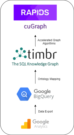
In this second part of our blog series, we take a deep dive into the use of graph algorithms with our GA360 SQL Knowledge Graph. We do so with RAPIDS cuGraph created by NVIDIA, a collection of powerful graph algorithms implemented over NVIDIA GPUs, leveraging our ability to analyze data at unmatched speeds.

RAPIDS cuGraph is paving the way in the graph world with multi-GPU graph analytics, allowing users to scale to billion and even trillion scale graphs, with performance speeds never seen before. cuGraph is equipped with many graph algorithms, falling into the following classes: Centrality, Community, Components, Core, Layout, Linear Assignment, Link Analysis, Link Prediction, Traversal, Structure, and other unique algorithms.

As there is a large rise in interest among companies to improve their analytics and boost their performance, many companies are turning to different graph options to get more out of their data. One of the main things holding companies back is the different implementation costs and barriers of adoption of these new technologies. Learning new languages to connect between your existing data infrastructure and new graph technologies is not only a headache but also a large expense.

This is where timbr comes into the picture. Timbr dramatically reduces implementation costs, as it does not require companies to transfer data or learn new languages. Instead, timbr acts as a virtual layer over the company’s existing data infrastructure, turning simple columns and tables into an easily accessible knowledge graph empowered with tools for exploration, visualization, and querying of data using graph algorithms. This is all delivered in a semantic SQL familiar to every analyst. 

In the blog post, we demonstrate the power of RAPIDS cuGraph combined with timbr by applying the Louvain Community Detection Algorithm as well as the Jaccard Similarity Algorithm on The GA360 SQL Knowledge Graph.

The Louvain Community Detection Algorithm

The Louvain community detection algorithm is used for detecting communities in large networks with a high density of connections, helping us uncover the different connections in a network. 

In order to understand the connections and be able to quantify their strength, we use what’s called modularity. Modularity is used to measure the strength of a partitioning of a graph into groups, clusters or communities, by constructing a score representing the modularity of a particular partitioning. The higher the modularity score, the denser the connections between the nodes in that community. 

Community detection is used today in many industries for many different reasons. The banking industry uses community detection for fraud analysis to find anomalies and evaluate whether a group has just a few discrete bad behaviors or is acting as a fraud ring. The health industry uses community detection to investigate different biological networks to identify various disease modules. The stock market uses community detection to build portfolios based on the correlation of stock prices.

So, with the many different uses of community detection that exist today, what can be done with community detection when it comes to Google Analytics? And how will it function when being used with RAPIDS cuGraph in comparison to the standard CPU in the form of NetworkX.

Let’s take a look:

After connecting our Google Analytics knowledge graph to cuGraph, we began with our first query requesting to see all the products purchased, allocated to their specific communities based on the customers who purchased these products. To run this query we used the gtimbr schema, which is timbr’s virtual schema for running graph algorithms. For the algorithm, we used the Louvain algorithm for community detection. 

Here is the exact query that was used:

SELECT id as productsku, community
FROM gtimbr.louvain(
 SELECT distinct productsku, info_of[hits].has_session[ga_sessions].fullvisitorid
 FROM dtimbr.product )

To understand the difference in performance when running this algorithm query, we tested running this query with cuGraph and then ran it again using NetworkX.

Here are the performance difference:

cuGraph vs NetworkX Performance Speeds

After running the query, we received a list of 982 products, each product belonging to a community ID.

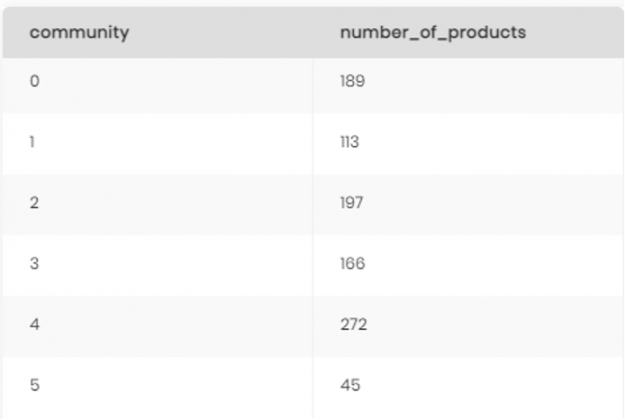
Having a large list of products, we needed to understand how many communities we were dealing with, so we ran the following query:

SELECT community, count(productsku) as number_of_products
FROM dtimbr.product_community
GROUP BY community
ORDER BY 1 asc

There were our results:

It was pretty clear from our results that having 982 products represented by just 6 communities makes it hard to understand the connections between the different products and customers. To resolve this, we decided to drill down into each community and create sub-communities to really highlight which products belong with which customers.

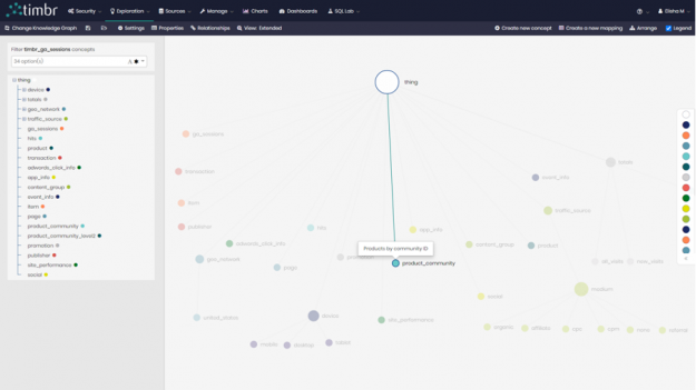
The first step was to simply create a new concept in the knowledge graph called product_community and map the data to it from our first query showing each of the 982 products and the community they belong to.

Mapping the data was then performed in simple SQL, similar to the syntax used when creating and mapping data with tables and columns in relational databases, and looked as follows:

CREATE OR REPLACE MAPPING map_product_community into product_community AS
 SELECT id as productsku, community
 FROM gtimbr.louvain(
       SELECT distinct productsku, info_of[hits].has_session[ga_sessions].fullvisitorid
       FROM dtimbr.product )

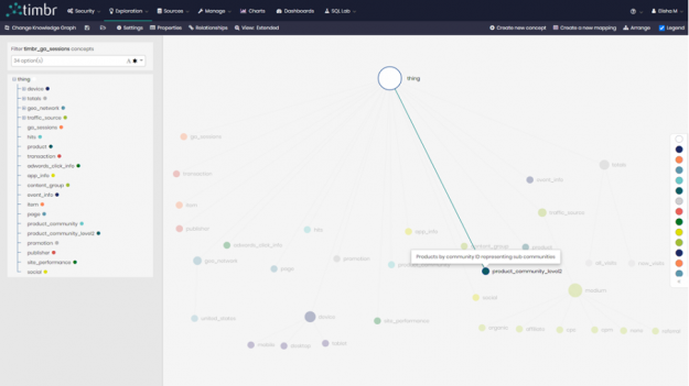
Now that we had a concept representing our products by the community, we created a second concept called product_community_level2 to represent the sub-communities of our original 6 communities.

To create the sub-communities for our new concept we created a new mapping for each of the 6 original communities. So for example, here is the new mapping to present the sub-communities for community ID “0”:

 CREATE OR REPLACE MAPPING map_product_community_level2_0 into product_community_level2 AS
 SELECT id as productsku, community, 0 as parent_community
 FROM gtimbr.louvain(
       SELECT distinct productsku, `info_of[hits].has_session[ga_sessions].fullvisitorid`
       FROM dtimbr.product
       WHERE productsku IN (SELECT distinct productsku
                            FROM dtimbr.product_community
                            WHERE community = 0))

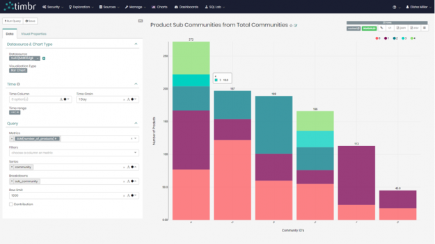
Once we queried and mapped the data of all the sub-communities to the new concept, we decided to view the results in our built-in BI Tool and created the following bar chart where we can clearly see the breakdown of the sub-communities for each of the original 6 communities:

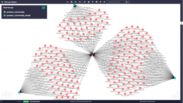
Lastly, we want to view the communities and sub-communities with all their products using timbr’s data explorer. We entered the concepts with the specific communities we wanted and asked to see their products. In this case, we asked for community numbers 0,1, and 4 as well as their sub-communities showing us products by sub-community within the larger community.

If we zoom in for example on community ID number “0”, we can see all the different product numbers appearing as pink nodes. Each product number is connected to the different sub-community that it belongs to, which appear as light blue nodes on the graph.

Link Prediction using Jaccard Similarity Algorithm

A variety of Similarity Algorithms are used today, algorithms such as Jaccard, Cosine, Pearson, Overlap, and others. In our GA Knowledge Graph, we demonstrate the use of the Jaccard similarity with an emphasis on link prediction.

The Jaccard similarity algorithm examines the similarity between different pairs and sets of items, whether it be people, products, or anything else. When using the similarity algorithm, we become exposed to connections between different pairs of people or items that we would have never been able to identify without the use of this unique algorithm.

The use of link prediction with similarity acts as a recommendation algorithm, which extends the idea of linkage measure to a recommendation in a bipartite network. In our case, a bipartite is a network of products and customers.

The Similarity Algorithm and link prediction are used today in many different use cases. Social networks use this algorithm for many different uses, including making recommendations to users regarding who to connect with based on similar relationships and connections, to deciding what advertisements to post for which users based on common interests with other users, all the way to offering a user a product based on the fact that the similarity algorithm matched him with a different user who bought that same product, which we will touch on shortly.

Governments use the algorithm to compare populations. Scientists use the algorithm to discover connections between different biological components, enabling them to safely develop new drugs, all the way to companies using the algorithm to advance their machine learning efforts and link prediction analysis.

So, now let’s apply similarity and link prediction in our Google Analytics Knowledge Graph empowered by NVIDIA’s cuGraph and witness its strength.

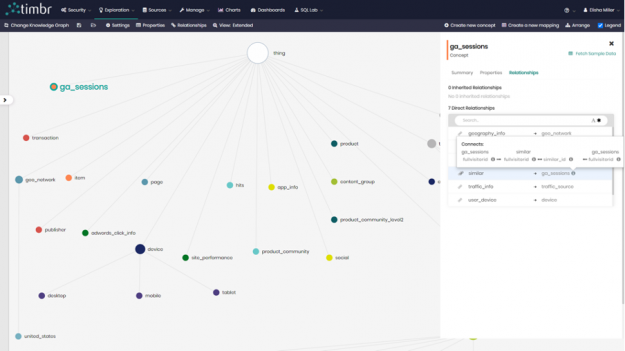
We began by creating a relationship called similar in our concept ga_sessions, a concept which contains data about all the sessions and visits of users to our website. Unlike in our example earlier on community detection, where we created a relationship between two concepts in our knowledge graph, here we decided to create a relationship between `ga_sessions` and itself, where the relationship would calculate the similarity between customers that searched for more than 1 similar keyword.

Once the relationship was created, it was time to map the data to the relationship. timbr allows us to not only map data to concepts but also to map data directly to relationships and extend them with their own properties (thus building a Property Graph).

The query we ran give us the similarity between customers that searched for more than 1 similar keyword, which we later mapped to our relationship similar in ga_session went as follows:

SELECT id as fullvisitorid, similar_id as similarid, similarity
FROM gtimbr.jaccard(
	SELECT `has_session[ga_sessions].fullvisitorid`, keyword
	FROM dtimbr.traffic_source
	WHERE `has_session[ga_sessions].fullvisitorid` in (
	-- Users that searched more than 1 keyword
		SELECT distinct `has_session[ga_sessions].fullvisitorid` as id
		FROM dtimbr.traffic_source
		WHERE keyword IS NOT NULL AND keyword != '(not provided)'
		GROUP BY `has_session[ga_sessions].fullvisitorid`
		HAVING count(1) > 1)
	AND keyword IS NOT NULL AND keyword != '(not provided)')

Once again, we compared the performance speeds running this algorithm query with cuGraph and NetworkX and received the following results:

cuGraph vs NetworkX Performance Speeds

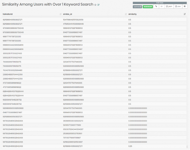
In the query, we asked for the fullvisitorid which is the user ID, the similar_id which returns IDs of similar users, as well as similarity which returns a Jaccard similarity score for each match of user IDs.

These were the results:

Next, we wanted to create a visualization using our similar relationship that we have created. We wrote the following query to do so:

SELECT DISTINCT  `fullvisitorid` AS user_id,
 `similar[ga_sessions].fullvisitorid` AS similar_user_id,
 `similar[ga_sessions]_similarity` AS similarity
FROM  dtimbr.ga_sessions
WHERE `similar[ga_sessions].fullvisitorid` IS NOT NULL

Now that we had all the visitor IDs and similar visitor ID’s that had more than 1 similar keyword, as well as _similarity where the underline before similarity represents the similarity score in the relationship, we were ready to visualize the results.

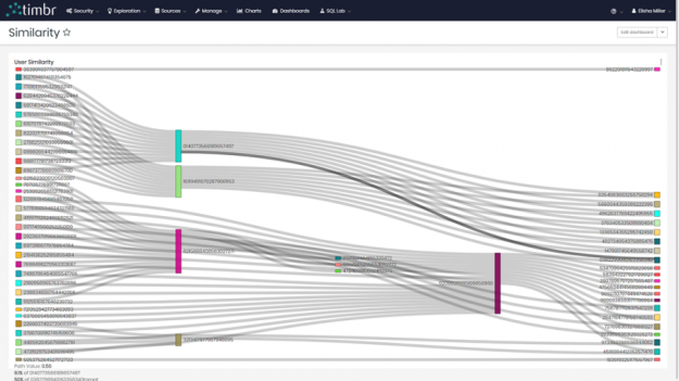
We decided to choose the Sankey Diagram to represent our findings.

We were able to see the different users on the left and right side connecting to their similar match in the middle. Many of these users both in the middle and on the sides connected to multiple users.

Combining the community and similarity algorithms

In our final example, we decided to build a recommendation query combing the relationships we’ve created for our community and similarity algorithms.

Here is the recommendation query:

SELECT similar[ga_sessions].has_hits[hits].ecommerce_product_data[product].productsku as productsku,
similar[ga_sessions].has_hits[hits].ecommerce_product_data[product].in_community[product_community].community AS community, 
COUNT(distinct similar[ga_sessions].fullvisitorid) num_of_users
FROM  dtimbr.ga_sessions
WHERE fullvisitorid = '9209808985108850988'
AND similar[ga_sessions].has_hits[hits].ecommerce_product_data[product].productsku is not null
GROUP BY similar[ga_sessions].has_hits[hits].ecommerce_product_data[product].productsku,  similar[ga_sessions].has_hits[hits].ecommerce_product_data[product].in_community[product_community].community
ORDER BY num_of_users DESC

What we did in this query, is we choose to focus on a random visitor with ID number ‘9209808985108850988’. We wanted the query to recommend products for our chosen user based on similar users who bought the recommended products. In order to gain more insight, we decided to ask for the communities that the recommended products belong to and see if there are any visible trends.

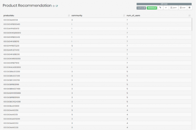
After running the query, the following results returned:

We were able to see the list of recommended products for user ID number ‘9209808985108850988’, and the community these products belong to, as well as the number of similar users to user ‘9209808985108850988’ who bought the specific product on the list.

Interestingly enough, the products recommended for user ‘9209808985108850988’ that have the most similar users who bought these products seem to largely fall in community ‘1’. If we were investigating further, this could have directed us to check whether it’s worth recommending user ‘9209808985108850988’ with more products belonging to community ‘1’.

Conclusion

We were able to demonstrate timbr’s advanced semantic capabilities using the Google Analytics Knowledge Graph combined with Graph Algorithms all in simple SQL, allowing us to analyze, explore and visualize our data. Not only were we able to perform in-depth analysis, but were able to do so with extremely high-performance speeds, going through large amounts of data in a matter of seconds.

We were able to accomplish our tasks and leverage our knowledge graph by connecting with RAPIDS cuGraph and NVIDIA GPU capabilities. Using cuGraph allowed us to query and analyze a mass amount of data in a fraction of the time it would have taken to do so using the standard CPU in NetworkX.

Click on timbr.ai and learn how you can leverage your data and performance speeds like never before.