So I have been working on a project, the model was trained on the screenshots that were taken on a laptop. When Images that are captured on a phone are fed to the model for testing the predictions are wrong, but when the same images are taken as screenshot[on a laptop] and fed to the model the predictions are correct. What is the issue here?
TensorFlow introduces the PluggableDevicearchitecture, which seamlessly integrates accelerators (GPUs, TPUs) with TensorFlow without making any changes in the TensorFlow code. PluggableDevice, as the name suggests, provides plug-in options for registering the devices with TensorFlow. It is constructed using the StreamExecutor C API and builds on the work done for Modular TensorFlow. In TF 2.5, the PluggableDevice feature is available.
I‘m a photographer and I have to crop a lot of pictures. I thought, I‘ll ask you guys. So I would need to identify the hips in order to crop the images. Tops in this situation. I have a bit of knowledge in Python. Is there an API or I have to install everything? Thank you.
“A confluence of advances has put us at the beginnings of the industrial HPC revolution,” said Jensen Huang. In a short talk viewable below, NVIDIA’s CEO described to a gathering of high performance computing specialists in Europe the genesis and outlook for the most powerful technology trend of our lifetimes. High performance computing is experiencing Read article >
NVIDIA’s 12th annual corporate social responsibility report, published today, shares our progress — and plans — to take care of employees, reach new sustainability goals and channel our tech to support the global community. Following a year of global hardship — the ongoing battle against the COVID-19 pandemic, social unrest and renewed calls for racial Read article >
Although ultrasound imaging is often used to detect breast cancer, especially mammographically occult cancers, its disadvantage is that it leads to high false-positive rates. We develop an AI system that achieves radiologist-level accuracy in identifying cancer. It is interpretable, achieves high accuracy on an external test set, and is trained in a weakly supervised manner.
Breast cancer is the most frequently diagnosed cancer among women worldwide. It’s also the leading cause of cancer-related deaths. Identifying breast cancer at an early stage before metastasis enables more effective treatments and therefore significantly improves survival rates.
Although mammography is the most widely used imaging technique for early detection of breast cancer, it is not always available in low-resource settings. Its sensitivity also drops for women with dense breast tissue.
Breast ultrasound is often used as a supplementary imaging modality to mammography in screening settings, and as the primary imaging modality in diagnostic settings. Despite its advantages, including lower costs relative to mammography, it is difficult to interpret breast ultrasound images as evident by the considerable intra-reader variability. This leads to increased false-positive findings, unnecessary biopsies, and significant discomfort to patients.
Previous work using deep learning for breast ultrasound has been based predominantly on small datasets on the scale of thousands of images. Many of these efforts also rely on expensive and time-consuming manual annotation of images to obtain image-level (presence of cancer in each image) or pixel-level (exact location of each lesion) labels.
Figure 1. Architecture of the deep neural network.
Radiologist diagnostic procedure compared to AI
The following table compares how radiologists make predictions compared to our AI system.
RADIOLOGIST
AI NETWORK
Looks for abnormal findings in each image within a breast ultrasound exam.
Processes each image within an exam independently using a ResNet-18 model and generates saliency map for it, indicating the most important parts.
Concentrates on images that contain suspicious lesions.
Assigns attention scores to each image based on its relative importance.
Considers signals in all images to make a final diagnosis
Aggregates information from all images using an attention mechanism to compute the final predictions for benign and malignant findings.
Table 1. Comparing radiology diagnostic procedure to AI
We compared the performance of the trained network to 10 board-certified breast radiologists in a reader study and to hybrid AI-radiologist models, which average the prediction of the AI and each radiologist.
The neural network was trained with a dataset consisting of approximately four million ultrasound images on an HPC cluster powered by NVIDIA technologies. The cluster consists of 34 computation nodes each of which is equipped with 80 CPUs and four NVIDIA V100 GPUs (16/32 GB). With this cluster, we performed hyperparameter search by launching experiments (each taking around 300 GPU hours) over a broad range of hyperparameters.
A large-scale dataset
Figure 2. Performance of the AI, readers, and hybrid models.
To complete this ambitious project, we preprocessed more than eight million breast ultrasound images collected at NYU Langone between 2012 and 2019 and extracted breast-level cancer labels by mining pathology reports.
Training set: 3,930,347 images within 209,162 exams collected from 101,493 patients.
Validation set: 653,924 images within 34,850 exams collected from 16,707 patients.
Internal test set: 858,636 images within 44,755 exams collected from 25,003 patients.
Results: the most exciting part!
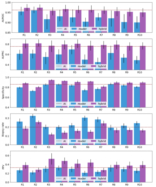
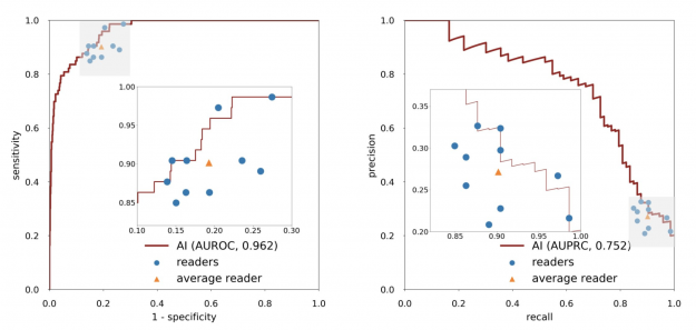
Our results show that a hybrid AI-radiologist model decreased false positive rates by 37.4% (that is, false suspicions of malignancy). This would lead to a reduction in the number of requested biopsies by 27.8%, while maintaining the same level of sensitivity as radiologists (Figure 3).
Figure 3. Performance of the AI compared to readers.
When acting independently, the AI system achieved higher area under the receiver operating characteristic curve (AUROC) and area under the precision recall curve (AUPRC) than individual readers. Figure 3 shows how each reader compares to the network’s performance.
Within the internal test set, the AI system maintained high diagnostic accuracy (0.940-0.990 AUROC) across all age groups, mammographic breast densities, and device manufacturers, including GE, Philips, and Siemens. In the biopsied population, it also achieved a 0.940 AUROC.
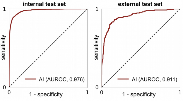
Figure 4. Performance across internal and external test sets
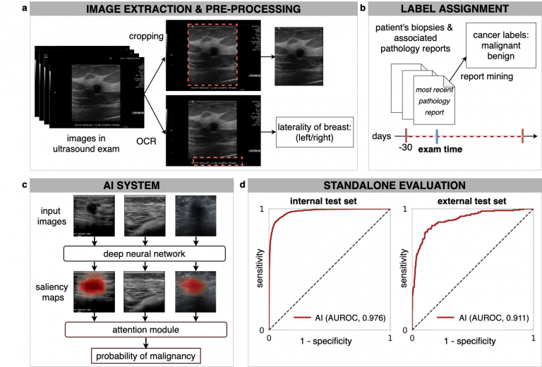
In an external test set collected in Egypt, the system achieved 0.911 AUROC, highlighting its generalization ability in patient demographics not seen during training (Figure 4).
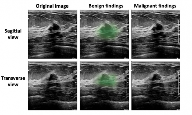
Based on qualitative assessment, the network produced appropriate localization information of benign and malignant lesions through its saliency maps. In the exam shown in Figure 4, all 10 breast radiologists thought the lesion appeared suspicious for malignancy and recommended that it undergo biopsy, while the AI system correctly classified it as benign. Most impressively, locations of lesions were never given during training, as it was trained in a weakly supervised manner!
Figure 5. Saliency maps produced by the network for benign (green) and malignant (red) findings.
Future work
For our next steps, we’d like to evaluate our system through prospective validation before it can be widely deployed in clinical practice. This enables us to measure its potential impact in improving the experience of women who undergo breast ultrasound examinations each year on a global level.
In conclusion, our work highlights the complementary role of an AI system in improving diagnostic accuracy by significantly decreasing unnecessary biopsies. Beyond improving radiologists’ performance, we have made technical contributions to the methodology of deep learning for medical imaging analysis.
JPEG 2000 (.jp2, .jpg2, .j2k) is an image compression standard defined by the Joint Photographers Expert Group (JPEG) as the more flexible successor to the still popular JPEG standard. Part 1 of the JPEG 2000 standard, which forms the core coding system, was first approved in August 2002. To date, the standard has expanded to … Continued
JPEG 2000 (.jp2, .jpg2, .j2k) is an image compression standard defined by the Joint Photographers Expert Group (JPEG) as the more flexible successor to the still popular JPEG standard. Part 1 of the JPEG 2000 standard, which forms the core coding system, was first approved in August 2002. To date, the standard has expanded to 17 parts, covering areas like Motion JPEG2000 (Part 3) which extends the standard for video, extensions for three-dimensional data (Part 10), and so on.
Features like mathematically lossless compression and large precision and higher dynamic range per component helped JPEG 2000 find adoption in digital cinema applications. JPEG 2000 is also widely used in digital pathology and geospatial imaging, where image dimensions exceed 4K but regions of interest (ROI) stay small.
GPU acceleration using the nvJPEG2000 library
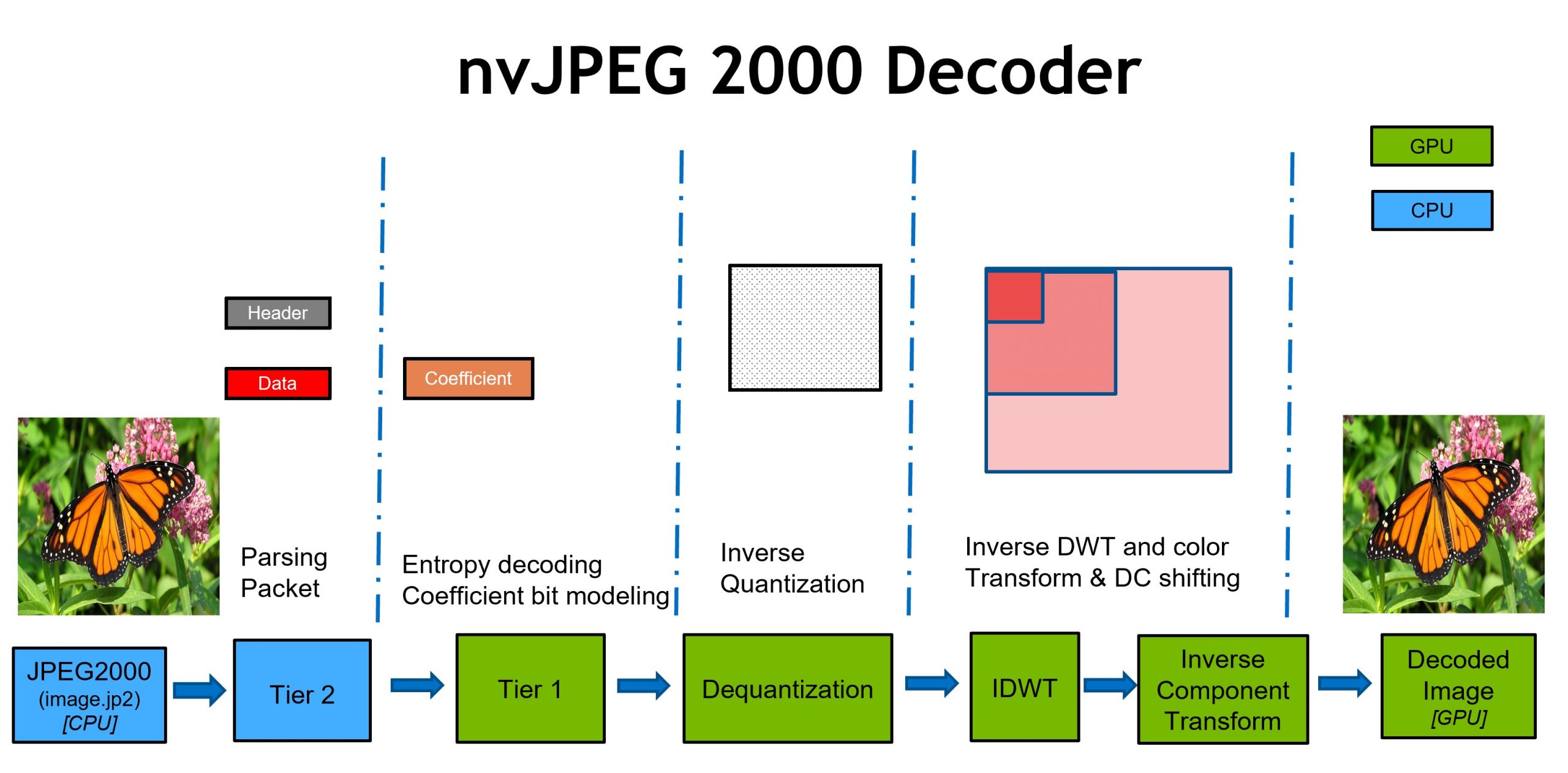
The JPEG 2000 feature set provides ample opportunities for GPU acceleration when compared to its predecessor, JPEG. Through GPU acceleration, images can be decoded in parallel and larger images can be processed quicker. nvJPEG2000 is a new library that accelerates the decoding of JPEG 2000 images on NVIDIA GPUs. It supports codec features commonly used in geospatial imaging, remote sensing, and digital pathology. Figure 1 overviews the decoding stages that nvJPEG2000 accelerates.
Figure 1. GPU-accelerated JPEG 2000 decode process. Stages run on the CPU are denoted by the first two blue boxes. All remaining stages are offloaded to the GPU as shown in green.
The Tier1 Decode (entropy decode) stage is the most compute-intensive stage of the entire decode process. The entropy decode algorithm used in the legacy JPEG codec was serial in nature and was hard to parallelize.
In JPEG 2000, the entropy decode stage is applied at a block-based granularity (typical block sizes are 64×64 and 32×32) that makes it possible to offload the entropy decode stage entirely to the GPU. For more information about the entropy decode process, see Section C of the JPEG 2000 Core coding system specification.
The JPEG 2000 core coding system allows for two types of wavelet transforms (5-3 Reversible and 9-7 Irreversible), both of which benefit from GPU acceleration. For more information about the wavelet transforms, see Section F of the JPEG 2000 Core coding system specification.
Decoding geospatial images
In this section, we concentrate on the new nvJPEG2000 API tailored for the geospatial domain, which enables decoding specific tiles within an image instead of decoding the full image.
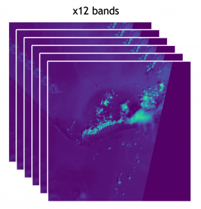
Figure 2. Sentinel2 Imaging (S2B_17RQK_20190908_0_L2A) JPEG2000 (Image Size 10980×10980, Tile Size 1024×1024, No of Tiles 11×11, Number of components 1).
Imaging data captured by the European Space Agency’s Sentinel 2 satellites are stored as JPEG 2000 bitstreams. Sentinel 2 level 2A data downloaded from the Copernicus hub can be used with the nvJPEG2000 decoding examples. The imaging data has 12 bands or channels and each of them is stored as an independent JPEG 2000 bitstream. The image in Figure 2 is subdivided into 121 tiles. To speed up the decode of multitile images, a new API called nvjpeg2kDecodeTile has been added in nvJPEG2000 v 0.2, which enables you to decode each tile independently.
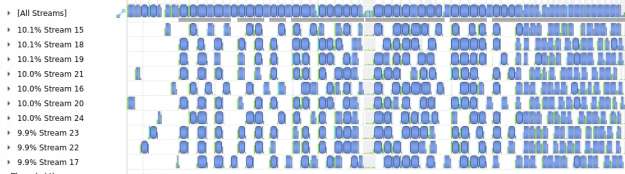
For multitile images, decoding each tile sequentially would be suboptimal. The GitHub multitile decode sample demonstrates how to decode each tile on a separate cudaStream_t. By taking this approach, you can simultaneously decode multiple tiles on the GPU. Nsight Systems trace in Figure 3 shows the decoding of Sentinel 2 data set consisting of 12 bands. By using 10 CUDA streams, up to 10 tiles are being decoded in parallel at any point during the decode process.
Figure 3. Nsight Systems trace demonstrating the decoding of multiple tiles on separate CUDA streams
Table 1 shows performance data comparing a single stream and multiple streams on a GV100 GPU.
# of CUDA streams
Average decode time (ms)
Speedup in % over single CUDA stream decode
1
0.888854
–
10
0.227408
75%
Table 1. Single stream vs multiple streams decode performance on a Quadro GV 100 for Sentinel2 Dataset
Using 10 CUDA streams reduces the total decode time of the entire dataset by about 75% on a Quadro GV100 GPU. For more information, see the Accelerating Geospatial Remote Sensing Workflows Using NVIDIA SDKs [S32150] GTC’21 talk. It discusses geospatial image-processing workflows in more detail and the role nvJPEG2000 plays there.
Decoding digital pathology images
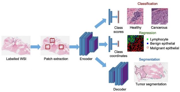
JPEG 2000 is used in digital pathology to store whole slide images (WSI). Figure 4 gives an overview of various deep learning techniques that can be applied to WSI. Deep learning models can be used to distinguish between cancerous and healthy cells. Image segmentation methods can be used to identify a tumor location in the WSI. For more information, see Deep neural network models for computational histopathology: A survey.
Figure 4. Digital pathology workflows
Table 2 lists the key parameters and their commonly used values of a whole slide image (WSI) compressed using JPEG 2000.
Image size
92000×201712
Tile size
92000×201712
# of tiles
1
# of components
3
Precision
8
Table 2. Key JPEG 2000 parameters and their values used in digital pathology.
The image in question is large and it is not possible to decode the entire image at one time due to the amount of memory required. The size of the decode output is around 53 GB (92000×201712 * 3). This is excluding the decoder memory requirements.
There are several approaches to handling such large images. In this post, we describe two of them:
Decoding an area of interest
Decoding the image at lower resolution
Both approaches can be easily performed using specific nvJPEG2000 APIs.
Decoding an area of interest in an image
The nvJPEG2000 library enables the decoding of a specific area of interest in an image supported as part of the nvjpeg2kDecodeTile API. The following code example shows how to set the area of interest in terms of image coordinates. The nvjpeg2kDecodeParams_t type enables you to control the decode output settings, such as the area of interest to decode.
 nvjpeg2kDecodeParams_t decode_params;
 // all coordinate values are relative to the top-left corner of the image
 uint32_t top_coordinate, bottom_coordinate, left_coordinate, right_coordinate;
 uint32_t tile_id;

 nvjpeg2kDecodeParamsSetDecodeArea(decode_params, left_coordinate, right_coordinate, top_coordinate, bottom_coordinate);

 nvjpeg2kDecodeTile(nvjpeg2k_handle, nvjpeg2k_decode_state,
                 jpeg2k_stream, decode_params, tile_id, 0,
                 &nvjpeg2k_out, cuda_stream)
For more information about how to partially decode an image with multiple tiles, see the Decode Tile Decode GitHub sample.
Decoding lower resolutions of an image
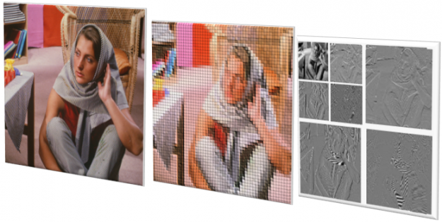
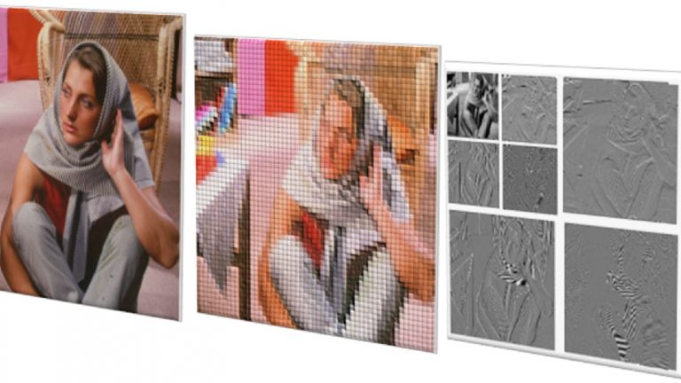
The second approach to decode a large image is to decode the image at lower resolutions. The ability to decode only the lower resolutions is a benefit of JPEG 2000 using wavelet transforms. In Figure 5, wavelet transform is applied up to two levels, which gives you access to the image at three resolutions. By controlling how the inverse wavelet transform is applied, you decode only the lower resolutions of an image.
Figure 5. Output of a 2D wavelet transform with two-level decomposition
The digital pathology image described in Table 2 has 12 resolutions. This information can be retrieved on a per-tile basis:
The image has a size of 92000×201712 with 12 resolutions. If you choose to discard the four higher resolutions and decode the image up to eight resolutions, that means you can extract an image of size 5750×12574. By dropping four higher resolutions, you are scaling the result by a factor of 16.
 uint32_t num_res_to_decode = 8;
 // if num_res_to_decode > num_res nvjpeg2kDecodeTile will return an INVALID //PARAMETER ERROR

 nvjpeg2kDecodeTile(nvjpeg2k_handle, nvjpeg2k_decode_state, jpeg2k_stream,
     decode_params, tile_id, num_res_to_decode, &nvjpeg2k_out, cuda_stream)
Performance benchmarks
To show the performance improvement that decoding JPEG2000 on GPU brings, compare GPU-based nvJPEG2000 with CPU-based OpenJPEG.
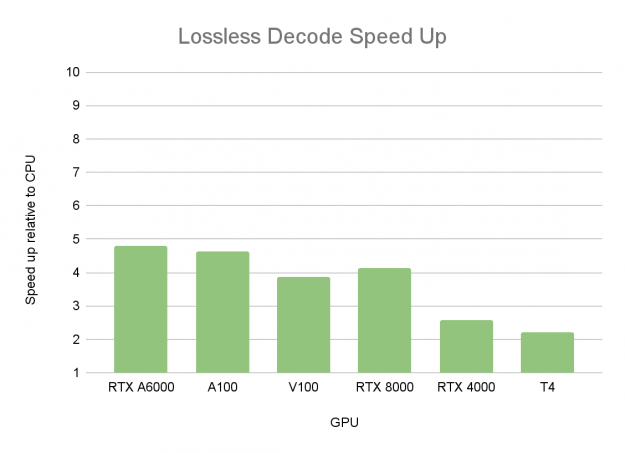
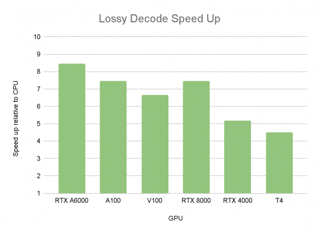
Figures 6 and 7 show the average speedup when decoding one image at a time. The following images are used in the measurements:
1920×1080 8-bit image with 444 chroma subsampling
3840×2160 8-bit image with 444 chroma subsampling
3328×4096 12-bit grayscale
Figure 6. Speed up for Lossless Decode (5-3 DWT) over CPU implementation using 16 threads.
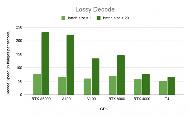
Figure 7. Speed for Lossy Decode (9-7 DWT) over CPU implementation using 16 threads
The tables were compiled with OpenJPEG CPU Performance – Intel Xeon Gold 6240@2GHz 3.9GHz Turbo (Cascade Lake) HT On, Number of CPU threads per image=16.
On NVIDIA Ampere Architecture GPUs such as NVIDIA RTX A6000, the speedup factor is more than 8x for decoding. This speedup is measured for single-image latency.
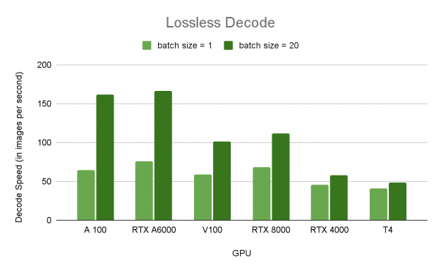
Even higher speedups can be achieved by batching the decode of multiple images. Figures 8 and 9 compare the speed of decoding a 1920×1080 8-bit image with 444 chroma subsampling (Full HD) in both lossless and lossy modes respectively across multiple GPUs.
Figure 8. Decode throughput comparison for a 1920×1080 8-bit 444 image using 5-3 wavelet transform (lossless decode).
Figure 9. Decode throughput comparison for a 1920×1080 8-bit 444 image using 9-7 wavelet transform (lossy decode).
Figures 8 and 9 demonstrate the benefits of batched decode using the nvJPEG2000 library. There’s a significant performance increase on GPUs with a large number of streaming multiprocessors (SMs), such as A100 and NVIDIA RTX A6000, than with smaller numbers of SMs, such as NVIDIA RTX 4000 and T4. By batching, you are making sure that the compute resources available are efficiently used.
As observed from Figure 8, the decode speed on an NVIDIA RTX A6000 is 232 images per second for a batch size of 20. This equates to an additional 3x speed over batch size = 1, based on a benchmark image with a low compression ratio. The compressed bitstream is only about 3x smaller than the uncompressed image. At higher compression ratios, the speedup is faster.
The following GitHub samples show how to achieve this speedup both at image and tile granularity:
The nvJPEG2000 library accelerates the decoding of JPEG2000 images both in size and volume using NVIDIA GPUs by targeting specific image-processing tasks of interest. Decoding JPEG 2000 images using the nvJPEG2000 library can be as much as 8x faster on GPU (NVIDIA RTX A6000) than on CPU. A further speedup of 3x (24x faster than CPU) is achieved by batching the decode of multiple images.
The simple nvJPEG2000 APIs make it easy to include in your applications and workflows. It is also integrated into the NVIDIA Data Loading Library (DALI), a data loading and preprocessing library to accelerate deep learning applications. Using nvJPEG2000 and DALI together makes it easy to use JPEG2000 images as part of deep learning training workflows.
For more information, see the following resources:
I have a YOLOv5 trained model converted to .tflite format having used this guide.
I use this code to print the input and output shape in python: “` interpreter = tf.lite.Interpreter( # model_path=”models/exported_resnet640.tflite”) # centernet_512x512 works correctly model_path=”models/yolov5_working.tflite”) # centernet_512x512 works correctly
Using the Tensorflow Lite c_api.h, I am trying to get the same output in C, but I cannot understand how to create the object that get the data.
I have tried using a float*** with size 1 * 14715 * 9 * sizeof(float) and get the output like so: “` int number_of_detections = 14175; struct filedata o_boxes; float **box_coords = (float *)malloc(sizeof(float *) * 1);
box_coords[0] = (float **)malloc(sizeof(float *) * (int)number_of_detections); for (int i = 0; i < (int)number_of_detections; i++) { box_coords[0][i] = (float *)calloc(sizeof(float), 9); // box has 9 coordinates }
for (int i = 0; i < o_boxes.size; i++) { for (int j = 0; j < 9; j++) { printf(“%f “, box_coords[0][i][j]); fflush(stdout); } printf(“n”); } where `struct filedata` is a simple struct: struct filedata { void *data; size_t size; }; “`
The result is some garbage big floats: 39688651931648.000000 0.000000 39805756899328.000000 0.000000 39807166185472.000000 0.000000 39807367512064.000000 0.000000 39807568838656.000000 and after the first iteration I get a Segmentation Fault.
How should I create/allocate my float array to get my data?
Hello, I’m trying to measure the performance (accuracy and loss) of my model and I discovered the evaluate() function for this.
My test data (34 pictures) is saved in a ‘test’ folder, so I tried to create an ImageDataGenerator and then to generate my data using flow_from_directory.
I receive a “Found 34 images belonging to 1 classes.” message. However, the result I get in the terminal for this code line result = seqModel.evaluate(data, batch_size=1, verbose=1) is a very weird one: 2/2 [==============================] – 0s 5ms/step – loss: 282.6923 – accuracy: 0.7353
Why do I receive a “2/2” everytime when running the script now, no matter what batch_size I choose? And why is my loss 282.6923, while accuracy is 0.7353? Doesn’t it look super weird? I know I’m doing something wrong, but I just can’t figure it out – maybe when creating the data generator or maybe when using flow_from_directory? (When I add the validationDataGenerator as first argument – in order to test it – it seems all fine, but here I just can’t figure it out.)


 Although ultrasound imaging is often used to detect breast cancer, especially mammographically occult cancers, its disadvantage is that it leads to high false-positive rates. We develop an AI system that achieves radiologist-level accuracy in identifying cancer. It is interpretable, achieves high accuracy on an external test set, and is trained in a weakly supervised manner.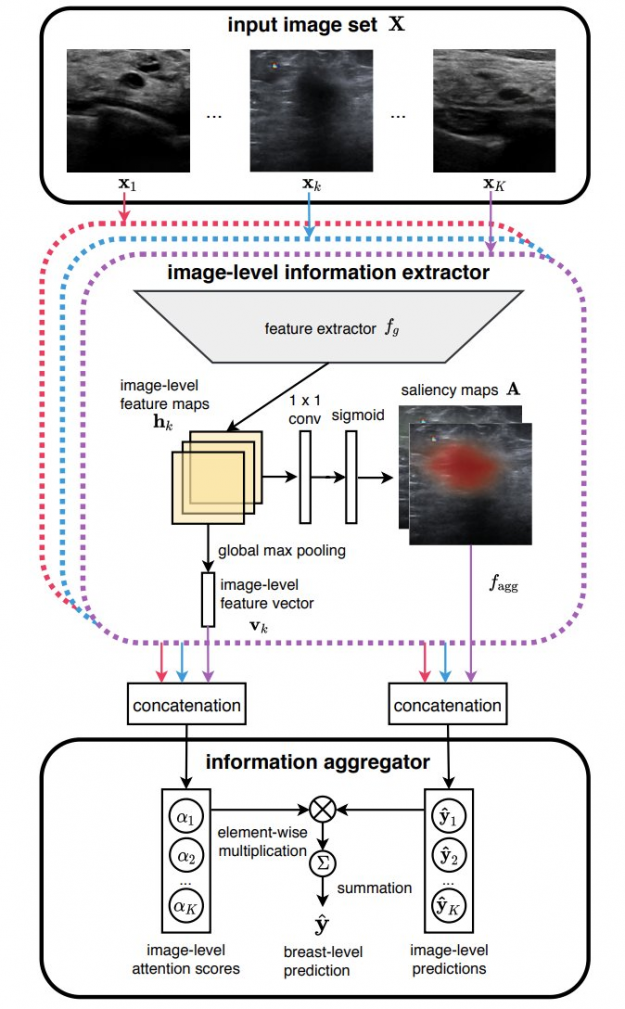
 JPEG 2000 (.jp2, .jpg2, .j2k) is an image compression standard defined by the Joint Photographers Expert Group (JPEG) as the more flexible successor to the still popular JPEG standard. Part 1 of the JPEG 2000 standard, which forms the core coding system, was first approved in August 2002. To date, the standard has expanded to …