Sparklyr 1.6 is now available on CRAN!
To install sparklyr 1.6 from CRAN, run
install.packages("sparklyr")
In this blog post, we shall highlight the following features and enhancements from sparklyr 1.6:
Weighted quantile summaries
Apache Spark is well-known for supporting approximate algorithms that trade off marginal amounts of accuracy for greater speed and parallelism. Such algorithms are particularly beneficial for performing preliminary data explorations at scale, as they enable users to quickly query certain estimated statistics within a predefined error margin, while avoiding the high cost of exact computations. One example is the Greenwald-Khanna algorithm for on-line computation of quantile summaries, as described in Greenwald and Khanna (2001). This algorithm was originally designed for efficient (epsilon)- approximation of quantiles within a large dataset without the notion of data points carrying different weights, and the unweighted version of it has been implemented as approxQuantile() since Spark 2.0. However, the same algorithm can be generalized to handle weighted inputs, and as sparklyr user @Zhuk66 mentioned in this issue, a weighted version of this algorithm makes for a useful sparklyr feature.
To properly explain what weighted-quantile means, we must clarify what the weight of each data point signifies. For example, if we have a sequence of observations ((1, 1, 1, 1, 0, 2, -1, -1)), and would like to approximate the median of all data points, then we have the following two options:
-
Either run the unweighted version of approxQuantile() in Spark to scan through all 8 data points
-
Or alternatively, “compress” the data into 4 tuples of (value, weight): ((1, 0.5), (0, 0.125), (2, 0.125), (-1, 0.25)), where the second component of each tuple represents how often a value occurs relative to the rest of the observed values, and then find the median by scanning through the 4 tuples using the weighted version of the Greenwald-Khanna algorithm
We can also run through a contrived example involving the standard normal distribution to illustrate the power of weighted quantile estimation in sparklyr 1.6. Suppose we cannot simply run qnorm() in R to evaluate the quantile function of the standard normal distribution at (p = 0.25) and (p = 0.75), how can we get some vague idea about the 1st and 3rd quantiles of this distribution? One way is to sample a large number of data points from this distribution, and then apply the Greenwald-Khanna algorithm to our unweighted samples, as shown below:
library(sparklyr)

sc <- spark_connect(master = "local")

num_samples <- 1e6
samples <- data.frame(x = rnorm(num_samples))

samples_sdf <- copy_to(sc, samples, name = random_string())

samples_sdf %>%
  sdf_quantile(
    column = "x",
    probabilities = c(0.25, 0.75),
    relative.error = 0.01
  ) %>%
  print()
##        25%        75%
## -0.6629242  0.6874939
Notice that because we are working with an approximate algorithm, and have specified relative.error = 0.01, the estimated value of (-0.6629242) from above could be anywhere between the 24th and the 26th percentile of all samples. In fact, it falls in the (25.36896)-th percentile:
pnorm(-0.6629242)
## [1] 0.2536896
Now how can we make use of weighted quantile estimation from sparklyr 1.6 to obtain similar results? Simple! We can sample a large number of (x) values uniformly randomly from ((-infty, infty)) (or alternatively, just select a large number of values evenly spaced between ((-M, M)) where (M) is approximately (infty)), and assign each (x) value a weight of (displaystyle frac{1}{sqrt{2 pi}}e^{-frac{x^2}{2}}), the standard normal distribution’s probability density at (x). Finally, we run the weighted version of sdf_quantile() from sparklyr 1.6, as shown below:
library(sparklyr)

sc <- spark_connect(master = "local")

num_samples <- 1e6
M <- 1000
samples <- tibble::tibble(
  x = M * seq(-num_samples / 2 + 1, num_samples / 2) / num_samples,
  weight = dnorm(x)
)

samples_sdf <- copy_to(sc, samples, name = random_string())

samples_sdf %>%
  sdf_quantile(
    column = "x",
    weight.column = "weight",
    probabilities = c(0.25, 0.75),
    relative.error = 0.01
  ) %>%
  print()
##    25%    75%
## -0.696  0.662
Voilà! The estimates are not too far off from the 25th and 75th percentiles (in relation to our abovementioned maximum permissible error of (0.01)):
pnorm(-0.696)
## [1] 0.2432144
pnorm(0.662)
## [1] 0.7460144
Power iteration clustering
Power iteration clustering (PIC), a simple and scalable graph clustering method presented in Lin and Cohen (2010), first finds a low-dimensional embedding of a dataset, using truncated power iteration on a normalized pairwise-similarity matrix of all data points, and then uses this embedding as the “cluster indicator”, an intermediate representation of the dataset that leads to fast convergence when used as input to k-means clustering. This process is very well illustrated in figure 1 of Lin and Cohen (2010) (reproduced below)
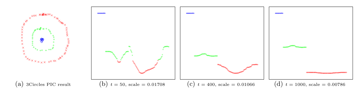
in which the leftmost image is the visualization of a dataset consisting of 3 circles, with points colored in red, green, and blue indicating clustering results, and the subsequent images show the power iteration process gradually transforming the original set of points into what appears to be three disjoint line segments, an intermediate representation that can be rapidly separated into 3 clusters using k-means clustering with (k = 3).
In sparklyr 1.6, ml_power_iteration() was implemented to make the PIC functionality in Spark accessible from R. It expects as input a 3-column Spark dataframe that represents a pairwise-similarity matrix of all data points. Two of the columns in this dataframe should contain 0-based row and column indices, and the third column should hold the corresponding similarity measure. In the example below, we will see a dataset consisting of two circles being easily separated into two clusters by ml_power_iteration(), with the Gaussian kernel being used as the similarity measure between any 2 points:
gen_similarity_matrix <- function() {
  # Guassian similarity measure
  guassian_similarity <- function(pt1, pt2) {
    exp(-sum((pt2 - pt1) ^ 2) / 2)
  }
  # generate evenly distributed points on a circle centered at the origin
  gen_circle <- function(radius, num_pts) {
    seq(0, num_pts - 1) %>%
      purrr::map_dfr(
        function(idx) {
          theta <- 2 * pi * idx / num_pts
          radius * c(x = cos(theta), y = sin(theta))
        })
  }
  # generate points on both circles
  pts <- rbind(
    gen_circle(radius = 1, num_pts = 80),
    gen_circle(radius = 4, num_pts = 80)
  )
  # populate the pairwise similarity matrix (stored as a 3-column dataframe)
  similarity_matrix <- data.frame()
  for (i in seq(2, nrow(pts)))
    similarity_matrix <- similarity_matrix %>%
      rbind(seq(i - 1L) %>%
        purrr::map_dfr(~ list(
          src = i - 1L, dst = .x - 1L,
          similarity = guassian_similarity(pts[i,], pts[.x,])
        ))
      )

  similarity_matrix
}

library(sparklyr)

sc <- spark_connect(master = "local")
sdf <- copy_to(sc, gen_similarity_matrix())
clusters <- ml_power_iteration(
  sdf, k = 2, max_iter = 10, init_mode = "degree",
  src_col = "src", dst_col = "dst", weight_col = "similarity"
)

clusters %>% print(n = 160)
## # A tibble: 160 x 2
##        id cluster
##     <dbl>   <int>
##   1     0       1
##   2     1       1
##   3     2       1
##   4     3       1
##   5     4       1
##   ...
##   157   156       0
##   158   157       0
##   159   158       0
##   160   159       0
The output shows points from the two circles being assigned to separate clusters, as expected, after only a small number of PIC iterations.
spark_write_rds() + collect_from_rds()
spark_write_rds() and collect_from_rds() are implemented as a less memory- consuming alternative to collect(). Unlike collect(), which retrieves all elements of a Spark dataframe through the Spark driver node, hence potentially causing slowness or out-of-memory failures when collecting large amounts of data, spark_write_rds(), when used in conjunction with collect_from_rds(), can retrieve all partitions of a Spark dataframe directly from Spark workers, rather than through the Spark driver node. First, spark_write_rds() will distribute the tasks of serializing Spark dataframe partitions in RDS version 2 format among Spark workers. Spark workers can then process multiple partitions in parallel, each handling one partition at a time and persisting the RDS output directly to disk, rather than sending dataframe partitions to the Spark driver node. Finally, the RDS outputs can be re-assembled to R dataframes using collect_from_rds().
Shown below is an example of spark_write_rds() + collect_from_rds() usage, where RDS outputs are first saved to HDFS, then downloaded to the local filesystem with hadoop fs -get, and finally, post-processed with collect_from_rds():
library(sparklyr)
library(nycflights13)

num_partitions <- 10L
sc <- spark_connect(master = "yarn", spark_home = "/usr/lib/spark")
flights_sdf <- copy_to(sc, flights, repartition = num_partitions)

# Spark workers serialize all partition in RDS format in parallel and write RDS
# outputs to HDFS
spark_write_rds(
  flights_sdf,
  dest_uri = "hdfs://<namenode>:8020/flights-part-{partitionId}.rds"
)

# Run `hadoop fs -get` to download RDS files from HDFS to local file system
for (partition in seq(num_partitions) - 1)
  system2(
    "hadoop",
    c("fs", "-get", sprintf("hdfs://<namenode>:8020/flights-part-%d.rds", partition))
  )

# Post-process RDS outputs
partitions <- seq(num_partitions) - 1 %>%
  lapply(function(partition) collect_from_rds(sprintf("flights-part-%d.rds", partition)))

# Optionally, call `rbind()` to combine data from all partitions into a single R dataframe
flights_df <- do.call(rbind, partitions)
Dplyr-related improvements
Similar to other recent sparklyr releases, sparklyr 1.6 comes with a number of dplyr-related improvements, such as
- Support for where() predicate within select() and summarize(across(…)) operations on Spark dataframes
- Addition of if_all() and if_any() functions
- Full compatibility with dbplyr 2.0 backend API
select(where(…)) and summarize(across(where(…)))
The dplyr where(…) construct is useful for applying a selection or aggregation function to multiple columns that satisfy some boolean predicate. For example,
library(dplyr)

iris %>% select(where(is.numeric))
returns all numeric columns from the iris dataset, and
library(dplyr)

iris %>% summarize(across(where(is.numeric), mean))
computes the average of each numeric column.
In sparklyr 1.6, both types of operations can be applied to Spark dataframes, e.g.,
library(dplyr)
library(sparklyr)

sc <- spark_connect(master = "local")
iris_sdf <- copy_to(sc, iris, name = random_string())

iris_sdf %>% select(where(is.numeric))

iris %>% summarize(across(where(is.numeric), mean))
if_all() and if_any()
if_all() and if_any() are two convenience functions from dplyr 1.0.4 (see here for more details) that effectively1 combine the results of applying a boolean predicate to a tidy selection of columns using the logical and/or operators.
Starting from sparklyr 1.6, if_all() and if_any() can also be applied to Spark dataframes, .e.g.,
library(dplyr)
library(sparklyr)

sc <- spark_connect(master = "local")
iris_sdf <- copy_to(sc, iris, name = random_string())

# Select all records with Petal.Width > 2 and Petal.Length > 2
iris_sdf %>% filter(if_all(starts_with("Petal"), ~ .x > 2))

# Select all records with Petal.Width > 5 or Petal.Length > 5
iris_sdf %>% filter(if_any(starts_with("Petal"), ~ .x > 5))
Compatibility with dbplyr 2.0 backend API
Sparklyr 1.6 is fully compatible with the newer dbplyr 2.0 backend API (by implementing all interface changes recommended in here), while still maintaining backward compatibility with the previous edition of dbplyr API, so that sparklyr users will not be forced to switch to any particular version of dbplyr.
This should be a mostly non-user-visible change as of now. In fact, the only discernible behavior change will be the following code
library(dbplyr)
library(sparklyr)

sc <- spark_connect(master = "local")

print(dbplyr_edition(sc))
outputting
[1] 2
if sparklyr is working with dbplyr 2.0+, and
[1] 1
if otherwise.
Acknowledgements
In chronological order, we would like to thank the following contributors for making sparklyr 1.6 awesome:
We would also like to give a big shout-out to the wonderful open-source community behind sparklyr, without whom we would not have benefitted from numerous sparklyr-related bug reports and feature suggestions.
Finally, the author of this blog post also very much appreciates the highly valuable editorial suggestions from @skeydan.
If you wish to learn more about sparklyr, we recommend checking out sparklyr.ai, spark.rstudio.com, and also some previous sparklyr release posts such as sparklyr 1.5 and sparklyr 1.4.
That is all. Thanks for reading!
Lin, Frank, and William Cohen. 2010. “Power Iteration Clustering.” In, 655–62.
-
modulo possible implementation-dependent short-circuit evaluations↩︎

 Learn from the world’s most advanced data science teams, here are some highlighted data science sessions planned for GTC.
 Developers are using the latest NVIDIA RTX technology to deliver the best gaming experience to players, complete with high-quality graphics and fast performance. But improving gameplay takes more than GPU power alone.
 NVIDIA CUDA-X AI are deep learning libraries for researchers and software developers to build high performance GPU-accelerated applications for conversational AI, recommendation systems and computer vision.
 Register for the free conference to hear talks from Audi Board Member Hildegard Wortmann, Zoox CTO Jesse Levinson, University of Toronto Professor Raquel Urtasun, and Cruise SVP of Engineering Mo ElShenawy.



 This tutorial is the sixth installment of introductions to the RAPIDS ecosystem.
 In this tutorial, we take a look at using Alluxio Data Orchestration across multiple stages of a data processing pipeline, from ETL to analytics and AI/ML.
 Learn how you can take advantage of the latest NVIDIA technology to enable the creation of beautiful worlds quicker and easier than ever before.