Category: Offsites

Posted by Chelsea Finn, Research Adviser and Eric Jang, Senior Research Scientist, Robotics at Google

People can flexibly maneuver objects in their physical surroundings to accomplish various goals. One of the grand challenges in robotics is to successfully train robots to do the same, i.e., to develop a general-purpose robot capable of performing a multitude of tasks based on arbitrary user commands. Robots that are faced with the real world will also inevitably encounter new user instructions and situations that were not seen during training. Therefore, it is imperative for robots to be trained to perform multiple tasks in a variety of situations and, more importantly, to be capable of solving new tasks as requested by human users, even if the robot was not explicitly trained on those tasks.

Existing robotics research has made strides towards allowing robots to generalize to new objects, task descriptions, and goals. However, enabling robots to complete instructions that describe entirely new tasks has largely remained out-of-reach. This problem is remarkably difficult since it requires robots to both decipher the novel instructions and identify how to complete the task without any training data for that task. This goal becomes even more difficult when a robot needs to simultaneously handle other axes of generalization, such as variability in the scene and positions of objects. So, we ask the question: How can we confer noteworthy generalization capabilities onto real robots capable of performing complex manipulation tasks from raw pixels? Furthermore, can the generalization capabilities of language models help support better generalization in other domains, such as visuomotor control of a real robot?

In “BC-Z: Zero-Shot Task Generalization with Robotic Imitation Learning”, published at CoRL 2021, we present new research that studies how robots can generalize to new tasks that they were not trained to do. The system, called BC-Z, comprises two key components: (i) the collection of a large-scale demonstration dataset covering 100 different tasks and (ii) a neural network policy conditioned on a language or video instruction of the task. The resulting system can perform at least 24 novel tasks, including ones that require interaction with pairs of objects that were not previously seen together. We are also excited to release the robot demonstration dataset used to train our policies, along with pre-computed task embeddings.

The BC-Z system allows a robot to complete instructions for new tasks that the robot was not explicitly trained to do. It does so by training the policy to take as input a description of the task along with the robot’s camera image and to predict the correct action.

Collecting Data for 100 Tasks
Generalizing to a new task altogether is substantially harder than generalizing to held-out variations in training tasks. Simply put, we want robots to have more generalization all around, which requires that we train them on large amounts of diverse data.

We collect data by teleoperating the robot with a virtual reality headset. This data collection follows a scheme similar to how one might teach an autonomous car to drive. First, the human operator records complete demonstrations of each task. Then, once the robot has learned an initial policy, this policy is deployed under close supervision where, if the robot starts to make a mistake or gets stuck, the operator intervenes and demonstrates a correction before allowing the robot to resume.

This mixture of demonstrations and interventions has been shown to significantly improve performance by mitigating compounding errors. In our experiments, we see a 2x improvement in performance when using this data collection strategy compared to only using human demonstrations.

Example demonstrations collected for 12 out of the 100 training tasks, visualized from the perspective of the robot and shown at 2x speed.

Training a General-Purpose Policy
For all 100 tasks, we use this data to train a neural network policy to map from camera images to the position and orientation of the robot’s gripper and arm. Crucially, to allow this policy the potential to solve new tasks beyond the 100 training tasks, we also input a description of the task, either in the form of a language command (e.g., “place grapes in red bowl”) or a video of a person doing the task.

To accomplish a variety of tasks, the BC-Z system takes as input either a language command describing the task or a video of a person doing the task, as shown here.

By training the policy on 100 tasks and conditioning the policy on such a description, we unlock the possibility that the neural network will be able to interpret and complete instructions for new tasks. This is a challenge, however, because the neural network needs to correctly interpret the instruction, visually identify relevant objects for that instruction while ignoring other clutter in the scene, and translate the interpreted instruction and perception into the robot’s action space.

Experimental Results
In language models, it is well known that sentence embeddings generalize on compositions of concepts encountered in training data. For instance, if you train a translation model on sentences like “pick up a cup” and “push a bowl”, the model should also translate “push a cup” correctly.

We study the question of whether the compositional generalization capabilities found in language encoders can be transferred to real robots, i.e., being able to compose unseen object-object and task-object pairs.

We test this method by pre-selecting a set of 28 tasks, none of which were among the 100 training tasks. For example, one of these new test tasks is to pick up the grapes and place them into a ceramic bowl, but the training tasks involve doing other things with the grapes and placing other items into the ceramic bowl. The grapes and the ceramic bowl never appeared in the same scene during training.

In our experiments, we see that the robot can complete many tasks that were not included in the training set. Below are a few examples of the robot’s learned policy.

The robot completes three instructions of tasks that were not in its training data, shown at 2x speed.

Quantitatively, we see that the robot can succeed to some degree on a total of 24 out of the 28 held-out tasks, indicating a promising capacity for generalization. Further, we see a notably small gap between the performance on the training tasks and performance on the test tasks. These results indicate that simply improving multi-task visuomotor control could considerably improve performance.

The BC-Z performance on held-out tasks, i.e., tasks that the robot was not trained to perform. The system correctly interprets the language command and translates that into action to complete many of the tasks in our evaluation.

Takeaways
The results of this research show that simple imitation learning approaches can be scaled in a way that enables zero-shot generalization to new tasks. That is, it shows one of the first indications of robots being able to successfully carry out behaviors that were not in the training data. Interestingly, language embeddings pre-trained on ungrounded language corpora make for excellent task conditioners. We demonstrated that natural language models can not only provide a flexible input interface to robots, but that pretrained language representations actually confer new generalization capabilities to the downstream policy, such as composing unseen object pairs together.

In the course of building this system, we confirmed that periodic human interventions are a simple but important technique for achieving good performance. While there is a substantial amount of work to be done in the future, we believe that the zero-shot generalization capabilities of BC-Z are an important advancement towards increasing the generality of robotic learning systems and allowing people to command robots. We have released the teleoperated demonstrations used to train the policy in this paper, which we hope will provide researchers with a valuable resource for future multi-task robotic learning research.

Acknowledgements
We would like to thank the co-authors of this research: Alex Irpan, Mohi Khansari, Daniel Kappler, Frederik Ebert, Corey Lynch, and Sergey Levine. This project was a collaboration between Google Research and the Everyday Robot Project. We would like to give special thanks to Noah Brown, Omar Cortes, Armando Fuentes, Kyle Jeffrey, Linda Luu, Sphurti Kirit More, Jornell Quiambao, Jarek Rettinghouse, Diego Reyes, Rosario Jau-regui Ruano, and Clayton Tan for overseeing robot operations and collecting human videos of the tasks, as well as Jeffrey Bingham, Jonathan Weisz, and Kanishka Rao for valuable discussions. We would also like to thank Tom Small for creating animations in this post and Paul Mooney for helping with dataset open-sourcing.

Posted by Alexey Kurakin, Software Engineer and Roxana Geambasu, Visiting Faculty Researcher, Google Research

Machine learning (ML) models are becoming increasingly valuable for improved performance across a variety of consumer products, from recommendations to automatic image classification. However, despite aggregating large amounts of data, in theory it is possible for models to encode characteristics of individual entries from the training set. For example, experiments in controlled settings have shown that language models trained using email datasets may sometimes encode sensitive information included in the training data and may have the potential to reveal the presence of a particular user’s data in the training set. As such, it is important to prevent the encoding of such characteristics from individual training entries. To these ends, researchers are increasingly employing federated learning approaches.

Differential privacy (DP) provides a rigorous mathematical framework that allows researchers to quantify and understand the privacy guarantees of a system or an algorithm. Within the DP framework, privacy guarantees of a system are usually characterized by a positive parameter ε, called the privacy loss bound, with smaller ε corresponding to better privacy. One usually trains a model with DP guarantees using DP-SGD, a specialized training algorithm that provides DP guarantees for the trained model.

However training with DP-SGD typically has two major drawbacks. First, most existing implementations of DP-SGD are inefficient and slow, which makes it hard to use on large datasets. Second, DP-SGD training often significantly impacts utility (such as model accuracy) to the point that models trained with DP-SGD may become unusable in practice. As a result most DP research papers evaluate DP algorithms on very small datasets (MNIST, CIFAR-10, or UCI) and don’t even try to perform evaluation of larger datasets, such as ImageNet.

In “Toward Training at ImageNet Scale with Differential Privacy”, we share initial results from our ongoing effort to train a large image classification model on ImageNet using DP while maintaining high accuracy and minimizing computational cost. We show that the combination of various training techniques, such as careful choice of the model and hyperparameters, large batch training, and transfer learning from other datasets, can significantly boost accuracy of an ImageNet model trained with DP. To substantiate these discoveries and encourage follow-up research, we are also releasing the associated source code.

Testing Differential Privacy on ImageNet
We choose ImageNet classification as a demonstration of the practicality and efficacy of DP because: (1) it is an ambitious task for DP, for which no prior work shows sufficient progress; and (2) it is a public dataset on which other researchers can operate, so it represents an opportunity to collectively improve the utility of real-life DP training. Classification on ImageNet is challenging for DP because it requires large networks with many parameters. This translates into a significant amount of noise added into the computation, because the noise added scales with the size of the model.

Scaling Differential Privacy with JAX
Exploring multiple architectures and training configurations to research what works for DP can be debilitatingly slow. To streamline our efforts, we used JAX, a high-performance computational library based on XLA that can do efficient auto-vectorization and just-in-time compilation of the mathematical computations. Using these JAX features was previously recommended as a good way to speed up DP-SGD in the context of smaller datasets such as CIFAR-10.

We created our own implementation of DP-SGD on JAX and benchmarked it against the large ImageNet dataset (the code is included in our release). The implementation in JAX was relatively simple and resulted in noticeable performance gains simply because of using the XLA compiler. Compared to other implementations of DP-SGD, such as that in Tensorflow Privacy, the JAX implementation is consistently several times faster. It is typically even faster compared to the custom-built and optimized PyTorch Opacus.

Each step of our DP-SGD implementation takes approximately two forward-backward passes through the network. While this is slower than non-private training, which requires only a single forward-backward pass, it is still the most efficient known approach to train with the per-example gradients necessary for DP-SGD. The graph below shows training runtimes for two models on ImageNet with DP-SGD vs. non-private SGD, each on JAX. Overall, we find DP-SGD on JAX sufficiently fast to run large experiments just by slightly reducing the number of training runs used to find optimal hyperparameters compared to non-private training. This is significantly better than alternatives, such as Tensorflow Privacy, which we found to be ~5x–10x slower on our CIFAR10 and MNIST benchmarks.

Time in seconds per training epoch on ImageNet using a Resnet18 or Resnet50 architecture with 8 V100 GPUs.

Combining Techniques for Improved Accuracy
It is possible that future training algorithms may improve DP’s privacy-utility tradeoff. However, with current algorithms, such as DP-SGD, our experience points to an engineering “bag-of-tricks” approach to make DP more practical on challenging tasks like ImageNet.

Because we can train models faster with JAX, we can iterate quickly and explore multiple configurations to find what works well for DP. We report the following combination of techniques as useful to achieve non-trivial accuracy and privacy on ImageNet:

• Full-batch training

  Theoretically, it is known that larger minibatch sizes improve the utility of DP-SGD, with full-batch training (i.e., where a full dataset is one batch) giving the best utility [1, 2], and empirical results are emerging to support this theory. Indeed, our experiments demonstrate that increasing the batch size along with the number of training epochs leads to a decrease in ε while still maintaining accuracy. However, training with extremely large batches is non-trivial as the batch cannot fit into GPU/TPU memory. So, we employed virtual large-batch training by accumulating gradients for multiple steps before updating the weights instead of applying gradient updates on each training step.

  Batch size		1024		4 × 1024		16 × 1024		64 × 1024
  Number of epochs		10		40		160		640
  Accuracy		56%		57.5%		57.9%		57.2%
  Privacy loss bound ε		9.8 × 108		6.1 × 107		3.5 × 106		6.7 × 104

• Transfer learning from public data

  Pre-training on public data followed by DP fine-tuning on private data has previously been shown to improve accuracy on other benchmarks [3, 4]. A question that remains is what public data to use for a given task to optimize transfer learning. In this work we simulate a private/public data split by using ImageNet as “private” data and using Places365, another image classification dataset, as a proxy for “public” data. We pre-trained our models on Places365 before fine-tuning them with DP-SGD on ImageNet. Places365 only has images of landscapes and buildings, not of animals as ImageNet, so it is quite different, making it a good candidate to demonstrate the ability of the model to transfer to a different but related domain.

  We found that transfer learning from Places365 gave us 47.5% accuracy on ImageNet with a reasonable level of privacy (ε = 10). This is low compared to the 70% accuracy of a similar non-private model, but compared to naïve DP training on ImageNet, which yields either very low accuracy (2 – 5%) or no privacy (ε=10⁹), this is quite good.

Privacy-accuracy tradeoff for Resnet-18 on ImageNet using large-batch training with transfer learning from Places365.

Next Steps
We hope these early results and source code provide an impetus for other researchers to work on improving DP for ambitious tasks such as ImageNet as a proxy for challenging production-scale tasks. With the much faster DP-SGD on JAX, we urge DP and ML researchers to explore diverse training regimes, model architectures, and algorithms to make DP more practical. To continue advancing the state of the field, we recommend researchers start with a baseline that incorporates full-batch training plus transfer learning.

Acknowledgments
This work was carried out with the support of the Google Visiting Researcher Program while Prof. Geambasu, an Associate Professor with Columbia University, was on sabbatical with Google Research. This work received substantial contributions from Steve Chien, Shuang Song, Andreas Terzis and Abhradeep Guha Thakurta.

Posted by Sungyong Seo, Software Engineer and Sercan O. Arik, Research Scientist, Google Research, Cloud AI Team

Deep neural networks (DNNs) provide more accurate results as the size and coverage of their training data increases. While investing in high-quality and large-scale labeled datasets is one path to model improvement, another is leveraging prior knowledge, concisely referred to as “rules” — reasoning heuristics, equations, associative logic, or constraints. Consider a common example from physics where a model is given the task of predicting the next state in a double pendulum system. While the model may learn to estimate the total energy of the system at a given point in time only from empirical data, it will frequently overestimate the energy unless also provided an equation that reflects the known physical constraints, e.g., energy conservation. The model fails to capture such well-established physical rules on its own. How could one effectively teach such rules so that DNNs absorb the relevant knowledge beyond simply learning from the data?

In “Controlling Neural Networks with Rule Representations”, published at NeurIPS 2021, we present Deep Neural Networks with Controllable Rule Representations (DeepCTRL), an approach used to provide rules for a model agnostic to data type and model architecture that can be applied to any kind of rule defined for inputs and outputs. The key advantage of DeepCTRL is that it does not require retraining to adapt the rule strength. At inference, the user can adjust rule strength based on the desired operation point of accuracy. We also propose a novel input perturbation method, which helps generalize DeepCTRL to non-differentiable constraints. In real-world domains where incorporating rules is critical — such as physics and healthcare — we demonstrate the effectiveness of DeepCTRL in teaching rules for deep learning. DeepCTRL ensures that models follow rules more closely while also providing accuracy gains at downstream tasks, thus improving reliability and user trust in the trained models. Additionally, DeepCTRL enables novel use cases, such as hypothesis testing of the rules on data samples and unsupervised adaptation based on shared rules between datasets.

The benefits of learning from rules are multifaceted:

• Rules can provide extra information for cases with minimal data, improving the test accuracy.
• A major bottleneck for widespread use of DNNs is the lack of understanding the rationale behind their reasoning and inconsistencies. By minimizing inconsistencies, rules can improve the reliability of and user trust in DNNs.
• DNNs are sensitive to slight input changes that are human-imperceptible. With rules, the impact of these changes can be minimized as the model search space is further constrained to reduce underspecification.

Learning Jointly from Rules and Tasks
The conventional approach to implementing rules incorporates them by including them in the calculation of the loss. There are three limitations of this approach that we aim to address: (i) rule strength needs to be defined before learning (thus the trained model cannot operate flexibly based on how much the data satisfies the rule); (ii) rule strength is not adaptable to target data at inference if there is any mismatch with the training setup; and (iii) the rule-based objective needs to be differentiable with respect to learnable parameters (to enable learning from labeled data).

DeepCTRL modifies canonical training by creating rule representations, coupled with data representations, which is the key to enable the rule strength to be controlled at inference time. During training, these representations are stochastically concatenated with a control parameter, indicated by α, into a single representation. The strength of the rule on the output decision can be improved by increasing the value of α. By modifying α at inference, users can control the behavior of the model to adapt to unseen data.

DeepCTRL pairs a data encoder and rule encoder, which produce two latent representations, which are coupled with corresponding objectives. The control parameter α is adjustable at inference to control the relative weight of each encoder.

Integrating Rules via Input Perturbations
Training with rule-based objectives requires the objectives to be differentiable with respect to the learnable parameters of the model. There are many valuable rules that are non-differentiable with respect to input. For example, “higher blood pressure than 140 is likely to lead to cardiovascular disease” is a rule that is hard to be combined with conventional DNNs. We also introduce a novel input perturbation method to generalize DeepCTRL to non-differentiable constraints by introducing small perturbations (random noise) to input features and constructing a rule-based constraint based on whether the outcome is in the desired direction.

Use Cases
We evaluate DeepCTRL on machine learning use cases from physics and healthcare, where utilization of rules is particularly important.

• Improved Reliability Given Known Principles in Physics

We quantify reliability of a model with the verification ratio, which is the fraction of output samples that satisfy the rules. Operating at a better verification ratio could be beneficial, especially if the rules are known to be always valid, as in natural sciences. By adjusting the control parameter α, a higher rule verification ratio, and thus more reliable predictions, can be achieved.

To demonstrate this, we consider the time-series data generated from double pendulum dynamics with friction from a given initial state. We define the task as predicting the next state of the double pendulum from the current state while imposing the rule of energy conservation. To quantify how much the rule is learned, we evaluate the verification ratio.

DeepCTRL enables controlling a model’s behavior after learning, but without retraining. For the example of a double pendulum, conventional learning imposes no constraints to ensure the model follows physical laws, e.g., conservation of energy. The situation is similar for the case of DeepCTRL where the rule strength is low. So, the total energy of the system predicted at time t+1 ( blue) can sometimes be greater than that measured at time t (red), which is physically disallowed (bottom left). If rule strength in DeepCTRL is high, the model may follow the given rule but lose accuracy (discrepancy between red and blue is larger; bottom right). If rule strength is between the two extremes, the model may achieve higher accuracy (blue curve is close to red) and follow the rule properly (blue curve is lower than red one).

We compare the performance of DeepCTRL on this task to conventional baselines of training with a fixed rule-based constraint as a regularization term added to the objective, λ. The highest of these regularization coefficients provides the highest verification ratio (shown by the green line in the second graph below), however, the prediction error is slightly worse than that of λ = 0.1 (orange line). We find that the lowest prediction error of the fixed baseline is comparable to that of DeepCTRL, but the highest verification ratio of the fixed baseline is still lower, which implies that DeepCTRL could provide accurate predictions while following the law of energy conservation. In addition, we consider the benchmark of imposing the rule-constraint with Lagrangian Dual Framework (LDF) and demonstrate two results where its hyperparameters are chosen by the lowest mean absolute error (LDF-MAE) and the highest rule verification ratio (LDF-Ratio) on the validation set. The performance of the LDF method is highly sensitive to what the main constraint is and its output is not reliable (black and pink dashed lines).

Experimental results for the double pendulum task, showing the task-based mean absolute error (MAE), which measures the discrepancy between the ground truth and the model prediction, versus DeepCTRL as a function of the control parameter α. TaskOnly doesn’t have a rule constraint and Task & Rule has different rule strength (λ). LDF enforces rules by solving a constraint optimization problem.

As above, but showing the verification ratio from different models.

Experimental results for the double pendulum task showing the current and predicted energy at time t and t + 1, respectively.

Additionally, the figures above illustrate the advantage DeepCTRL has over conventional approaches. For example, increasing the rule strength λ from 0.1 to 1.0 improves the verification ratio (from 0.7 to 0.9), but does not improve the mean absolute error. Arbitrarily increasing λ will continue to drive the verification ratio closer to 1, but will result in worse accuracy. Thus, finding the optimal value of λ will require many training runs through the baseline model, whereas DeepCTRL can find the optimal value for the control parameter α much more quickly.

• Adapting to Distribution Shifts in Healthcare

The strengths of some rules may differ between subsets of the data. For example, in disease prediction, the correlation between cardiovascular disease and higher blood pressure is stronger for older patients than younger patients. In such situations, when the task is shared but data distribution and the validity of the rule differ between datasets, DeepCTRL can adapt to the distribution shifts by controlling α.

Exploring this example, we focus on the task of predicting whether cardiovascular disease is present or not using a cardiovascular disease dataset. Given that higher systolic blood pressure is known to be strongly associated with cardiovascular disease, we consider the rule: “higher risk if the systolic blood pressure is higher”. Based on this, we split the patients into two groups: (1) unusual, where a patient has high blood pressure, but no disease or lower blood pressure, but has disease; and (2) usual, where a patient has high blood pressure and disease or low blood pressure, but no disease.

We demonstrate below that the source data do not always follow the rule, and thus the effect of incorporating the rule can depend on the source data. The test cross entropy, which indicates classification accuracy (lower cross entropy is better), vs. rule strength for source or target datasets with varying usual / unusual ratio are visualized below. The error monotonically increases as α → 1 because the enforcement of the imposed rule, which doesn’t accurately reflect the source data, becomes more strict.

Test cross entropy vs. rule strength for a source dataset with usual / unusual ratio of 0.30.

When a trained model is transferred to the target domain, the error can be reduced by controlling α. To demonstrate this, we show three domain-specific datasets, which we call Target 1, 2, and 3. In Target 1, where the majority of patients are from the usual group, as α is increased, the rule-based representation has more weight and the resultant error decreases monotonically.

As above, but for a Target dataset (1) with a usual / unusual ratio of 0.77.

When the ratio of usual patients is decreased in Target 2 and 3, the optimal α is an intermediate value between 0 and 1. These demonstrate the capability to adapt the trained model via α.

As above, but for Target 2 with a usual / unusual ratio of 0.50.

As above, but for Target 3 with a usual / unusual ratio of 0.40.

Conclusions
Learning from rules can be crucial for constructing interpretable, robust, and reliable DNNs. We propose DeepCTRL, a new methodology used to incorporate rules into data-learned DNNs. DeepCTRL enables controllability of rule strength at inference without retraining. We propose a novel perturbation-based rule encoding method to integrate arbitrary rules into meaningful representations. We demonstrate three use cases of DeepCTRL: improving reliability given known principles, examining candidate rules, and domain adaptation using the rule strength.

Acknowledgements
We greatly appreciate the contributions of Jinsung Yoon, Xiang Zhang, Kihyuk Sohn and Tomas Pfister.

Posted by Abhijit Guha Roy, Research Software Engineer and Jie Ren, Research Scientist, Google Research

Deep machine learning (ML) systems have achieved considerable success in medical image analysis in recent years. One major contributing factor is access to abundant labeled datasets, which are used to train highly effective supervised deep learning models. However, in the real-world, these models may encounter samples exhibiting rare conditions that are individually too infrequent for per-condition classification. Nevertheless, such conditions can be collectively common because they follow a long-tail distribution and when taken together can represent a significant portion of cases — e.g., in a recent deep learning dermatological study, hundreds of rare conditions composed around 20% of cases encountered by the model at test time.

To prevent models from generating erroneous outputs on rare samples at test time, there remains a considerable need for deep learning systems with the ability to recognize when a sample is not a condition it can identify. Detecting previously unseen conditions can be thought of as an out-of-distribution (OOD) detection task. By successfully identifying OOD samples, preventive measures can be taken, like abstaining from prediction or deferring to a human expert.

Traditional computer vision OOD detection benchmarks work to detect dataset distribution shifts. For example, a model may be trained on CIFAR images but be presented with street view house numbers (SVHN) as OOD samples, two datasets with very different semantic meanings. Other benchmarks seek to detect slight differences in semantic information, e.g., between images of a truck and a pickup truck, or two different skin conditions. The semantic distribution shifts in such near-OOD detection problems are more subtle in comparison to dataset distribution shifts, and thus, are harder to detect.

In “Does Your Dermatology Classifier Know What it Doesn’t Know? Detecting the Long-Tail of Unseen Conditions”, published in Medical Image Analysis, we tackle this near-OOD detection task in the application of dermatology image classification. We propose a novel hierarchical outlier detection (HOD) loss, which leverages existing fine-grained labels of rare conditions from the long tail and modifies the loss function to group unseen conditions and improve identification of these near OOD categories. Coupled with various representation learning methods and the diverse ensemble strategy, this approach enables us to achieve better performance for detecting OOD inputs.

The Near-OOD Dermatology Dataset
We curated a near-OOD dermatology dataset that includes 26 inlier conditions, each of which are represented by at least 100 samples, and 199 rare conditions considered to be outliers. Outlier conditions can have as low as one sample per condition. The separation criteria between inlier and outlier conditions can be specified by the user. Here the cutoff sample size between inlier and outlier was 100, consistent with our previous study. The outliers are further split into training, validation, and test sets that are intentionally mutually exclusive to mimic real-world scenarios, where rare conditions shown during test time may have not been seen in training.

Long tail distribution of different dermatological conditions in our dataset. The 26 inlier conditions, with at least 100 samples, (blue) and the remaining 199 rare outlier conditions (orange). Outlier conditions can have as low as one sample per condition.

	Train set		Validation set		Test set
	Inlier	Outlier	Inlier	Outlier	Inlier	Outlier
Number of classes	26	68	26	66	26	65
Number of samples	8854	1111	1251	1082	1192	937

Inlier and outlier conditions in our benchmark dataset and detailed dataset split statistics. The outliers are further split into mutually exclusive train, validation, and test sets.

Hierarchical Outlier Detection Loss
We propose to use “known outlier” samples during training that are leveraged to aid detection of “unknown outlier” samples during test time. Our novel hierarchical outlier detection (HOD) loss performs a fine-grained classification of individual classes for all inlier or outlier classes and, in parallel, a coarse-grained binary classification of inliers vs. outliers in a hierarchical setup (see the figure below). Our experiments confirmed that HOD is more effective than performing a coarse-grained classification followed by a fine-grained classification, as this could result in a bottleneck that impacted the performance of the fine-grained classifier.

We use the sum of the predictive probabilities of the outlier classes as the OOD score. As a primary OOD detection metric we use the area under receiver operating characteristics (AUROC) curve, which ranges between 0 and 1 and gives us a measure of separability between inliers and outliers. A perfect OOD detector, which separates all inliers from outliers, is assigned an AUROC score of 1. A popular baseline method, called reject bucket, separates each inlier individually from the outliers, which are grouped into a dedicated single abstention class. In addition to a fine-grained classification for each individual inlier and outlier classes, the HOD loss–based approach separates the inliers collectively from the outliers with a coarse-grained prediction loss, resulting in better generalization. While similar, we demonstrate that our HOD loss–based approach outperforms other baseline methods that leverage outlier data during training, achieving an AUROC score of 79.4% on the benchmark, a significant improvement over that of reject bucket, which achieves 75.6%.

Our model architecture and the HOD loss. The encoder (green) represents the wide ResNet 101×3 model pre-trained with different representation learning models (ImageNet, BiT, SimCLR, and MICLe; see below). The output of the encoder is sent to the HOD loss where fine-grained and coarse-grained predictions for inliers (blue) and outliers (orange) are obtained. The coarse predictions are obtained by summing over the fine-grained probabilities as indicated in the figure. The OOD score is defined as the sum of the probabilities of outlier classes.

Representation Learning and the Diverse Ensemble Strategy
We also investigate how different types of representation learning help in OOD detection in conjunction with HOD by pretraining on ImageNet, BiT-L, SimCLR and MICLe models. We observe that including HOD loss improves OOD performance compared to the reject bucket baseline method for all four representation learning methods.

Representation Learning Methods	OOD detection metric (AUROC %)
	With reject bucket	With HOD loss
ImageNet	74.7%	77%
BiT-L	75.6%	79.4%
SimCLR	75.2%	77.2%
MICLe	76.7%	78.8%

OOD detection performance for different representation learning models with reject bucket and with HOD loss.

Another orthogonal approach for improving OOD detection performance and accuracy is deep ensemble, which aggregates outputs from multiple independently trained models to provide a final prediction. We build upon deep ensemble, but instead of using a fixed architecture with a fixed pre-training, we combine different representation learning architectures (ImageNet, BiT-L, SimCLR and MICLe) and introduce objective loss functions (HOD and reject bucket). We call this a diverse ensemble strategy, which we demonstrate outperforms the deep ensemble for OOD performance and inlier accuracy.

Downstream Clinical Trust Analysis
While we mainly focus on improving the performance for OOD detection, the ultimate goal for our dermatology model is to have high accuracy in predicting inlier and outlier conditions. We go beyond traditional performance metrics and introduce a “penalty” matrix that jointly evaluates inlier and outlier predictions for model trust analysis to approximate downstream impact. For a fixed confidence threshold, we count the following types of mistakes: (i) incorrect inlier predictions (i.e., mistaking inlier condition A as inlier condition B); (ii) incorrect abstention of inliers (i.e., abstaining from making a prediction for an inlier); and (iii) incorrect prediction for outliers as one of the inlier classes.

To account for the asymmetrical consequences of the different types of mistakes, penalties can be 0, 0.5, or 1. Both incorrect inlier and outlier-as-inlier predictions can potentially erode user trust in the model and were penalized with a score of 1. Incorrect abstention of an inlier as an outlier was penalized with a score of 0.5, indicating that potential model users should seek additional guidance given the model-expressed uncertainty or abstention. For correct decisions no cost is incurred, indicated by a score of 0.

	Action of the Model
	Prediction as Inlier	Abstain
Inlier	0 (Correct) 1 (Incorrect, mistakes that may erode trust)	0.5 (Incorrect, abstains inliers)
Outlier	1 (Incorrect, mistakes that may erode trust)	0 (Correct)

The penalty matrix is designed to capture the potential impact of different types of model errors.

Because real-world scenarios are more complex and contain a variety of unknown variables, the numbers used here represent simplifications to enable qualitative approximations for the downstream impact on user trust of outlier detection models, which we refer to as “cost”. We use the penalty matrix to estimate a downstream cost on the test set and compare our method against the baseline, thereby making a stronger case for its effectiveness in real-world scenarios. As shown in the plot below, our proposed solution incurs a much lower estimated cost in comparison to baseline over all possible operating points.

Trust analysis comparing our proposed method to the baseline (reject bucket) for a range of outlier recall rates, indicated by 𝛕. We show that our method reduces downstream estimated cost, potentially reflecting improved downstream impact.

Conclusion
In real-world deployment, medical ML models may encounter conditions that were not seen in training, and it’s important that they accurately identify when they do not know a specific condition. Detecting those OOD inputs is an important step to improving safety. We develop an HOD loss that leverages outlier data during training, and combine it with pre-trained representation learning models and a diverse ensemble to further boost performance, significantly outperforming the baseline approach on our new dermatology benchmark dataset. We believe that our approach, aligned with our AI Principles, can aid successful translation of ML algorithms into real-world scenarios. Although we have primarily focused on OOD detection for dermatology, most of our contributions are fairly generic and can be easily incorporated into OOD detection for other applications.

Acknowledgements
We would like to thank Shekoofeh Azizi, Aaron Loh, Vivek Natarajan, Basil Mustafa, Nick Pawlowski, Jan Freyberg, Yuan Liu, Zach Beaver, Nam Vo, Peggy Bui, Samantha Winter, Patricia MacWilliams, Greg S. Corrado, Umesh Telang, Yun Liu, Taylan Cemgil, Alan Karthikesalingam, Balaji Lakshminarayanan, and Jim Winkens for their contributions. We would also like to thank Tom Small for creating the post animation.

Posted by Matt McEwen, Student Researcher, Google Quantum AI and Lara Faoro, Research Fellow, LPTHE- Sorbonne Université and CNRS (Paris)

Quantum processors are made of superconducting quantum bits (qubits) that — being quantum objects — are highly susceptible to even tiny amounts of environmental noise. This noise can cause errors in quantum computation that need to be addressed to continue advancing quantum computers. Our Sycamore processors are installed in specially designed cryostats, where they are sealed away from stray light and electromagnetic fields and are cooled down to very low temperatures to reduce thermal noise.

However, the world is full of high-energy radiation. In fact, there’s a tiny background of high-energy gamma rays and muons that pass through everything around us all the time. While these particles interact so weakly that they don’t cause any harm in our day-to-day lives, qubits are sensitive enough that even weak particle interactions can cause significant interference.

In “Resolving Catastrophic Error Bursts from Cosmic Rays in Large Arrays of Superconducting Qubits”, published in Nature Physics, we identify the effects of these high-energy particles when they impact the quantum processor. To detect and study individual impact events, we use new techniques in rapid, repetitive measurement to operate our processor like a particle detector. This allows us to characterize the resulting burst of errors as they spread through the chip, helping to better understand this important source of correlated errors.

The Dynamics of a High-Energy Impact
The Sycamore quantum processor is constructed with a very thin layer of superconducting aluminum on a silicon substrate, onto which a pattern is etched to define the qubits. At the center of each qubit is the Josephson junction, a superconducting component that defines the distinct energy levels of the qubit, which are used for computation. In a superconducting metal, electrons bind together into a macroscopic, quantum state, which allows electrons to flow as a current with zero resistance (a supercurrent). In superconducting qubits, information is encoded in different patterns of oscillating supercurrent going back and forth through the Josephson junction.

If enough energy is added to the system, the superconducting state can be broken up to produce quasiparticles. These quasiparticles are a problem, as they can absorb energy from the oscillating supercurrent and jump across the Josephson junction, which changes the qubit state and produces errors. To prevent any energy from being absorbed by the chip and producing quasiparticles, we use extensive shielding for electric and magnetic fields, and powerful cryogenic refrigerators to keep the chip near absolute zero temperature, thus minimizing the thermal energy.

A source of energy that we can’t effectively shield against is high-energy radiation, which includes charged particles and photons that can pass straight through most materials. One source of these particles are tiny amounts of radioactive elements that can be found everywhere, e.g., in building materials, the metal that makes up our cryostats, and even in the air. Another source is cosmic rays, which are extremely energetic particles produced by supernovae and black holes. When cosmic rays impact the upper atmosphere, they create a shower of high-energy particles that can travel all the way down to the surface and through our chip. Between radioactive impurities and cosmic ray showers, we expect a high energy particle to pass through a quantum chip every few seconds.

When a high-energy impact event occurs, energy spreads through the chip in the form of phonons. When these arrive at the superconducting qubit layer, they break up the superconducting state and produce quasiparticles, which cause the qubit errors we observe.

When one of these particles impinges on the chip, it passes straight through and deposits a small amount of its energy along its path through the substrate. Even a small amount of energy from these particles is a very large amount of energy for the qubits. Regardless of where the impact occurs, the energy quickly spreads throughout the entire chip through quantum vibrations called phonons. When these phonons hit the aluminum layer that makes up the qubits, they have more than enough energy to break the superconducting state and produce quasiparticles. So many quasiparticles are produced that the probability of the qubits interacting with one becomes very high. We see this as a sudden and significant increase in errors over the whole chip as those quasiparticles absorb energy from the qubits. Eventually, as phonons escape and the chip cools, these quasiparticles recombine back into the superconducting state, and the qubit error rates slowly return to normal.

A high-energy particle impact (at time = 0 ms) on a patch of the quantum processor, showing error rates for each qubit over time. The event starts by rapidly spreading error over the whole chip, before saturating and then slowly returning to equilibrium.

Detecting Particles with a Computer
The Sycamore processor is designed to perform quantum error correction (QEC) to improve the error rates and enable it to execute a variety of quantum algorithms. QEC provides an effective way of identifying and mitigating errors, provided they are sufficiently rare and independent. However, in the case of a high-energy particle going through the chip, all of the qubits will experience high error rates until the event cools off, producing a correlated error burst that QEC won’t be able to correct. In order to successfully perform QEC, we first have to understand what these impact events look like on the processor, which requires operating it like a particle detector.

To do so, we take advantage of recent advances in qubit state preparation and measurement to quickly prepare each qubit in their excited state, similar to flipping a classical bit from 0 to 1. We then wait for a short idle time and measure whether they are still excited. If the qubits are behaving normally, almost all of them will be. Further, the qubits that experience a decay out of their excited state won’t be correlated, meaning the qubits that have errors will be randomly distributed over the chip.

However, during the experiment we occasionally observe large error bursts, where all the qubits on the chip suddenly become more error prone all at once. This correlated error burst is a clear signature of a high-energy impact event. We also see that, while all qubits on the chip are affected by the event, the qubits with the highest error rates are all concentrated in a “hotspot” around the impact site, where slightly more energy is deposited into the qubit layer by the spreading phonons.

To detect high-energy impacts, we rapidly prepare the qubits in an excited state, wait a little time, and then check if they’ve maintained their state. An impact produces a correlated error burst, where all the qubits show a significantly elevated error rate, as shown around time = 8 seconds above.

Next Steps
Because these error bursts are severe and quickly cover the whole chip, they are a type of correlated error that QEC is unable to correct. Therefore, it’s very important to find a solution to mitigate these events in future processors that are expected to rely on QEC.

Shielding against these particles is very difficult and typically requires careful engineering and design of the cryostat and many meters of shielding, which becomes more impractical as processors grow in size. Another approach is to modify the chip, allowing it to tolerate impacts without causing widespread correlated errors. This is an approach taken in other complex superconducting devices like detectors for astronomical telescopes, where it’s not possible to use shielding. Examples of such mitigation strategies include adding additional metal layers to the chip to absorb phonons and prevent them from getting to the qubit, adding barriers in the chip to prevent phonons spreading over long distances, and adding traps for quasiparticles in the qubits themselves. By employing these techniques, future processors will be much more robust to these high-energy impact events.

As the error rates of quantum processors continue to decrease, and as we make progress in building a prototype of an error-corrected logical qubit, we’re increasingly pushed to study more exotic sources of error. While QEC is a powerful tool for correcting many kinds of errors, understanding and correcting more difficult sources of correlated errors will become increasingly important. We’re looking forward to future processor designs that can handle high energy impacts and enable the first experimental demonstrations of working quantum error correction.

Acknowledgements
This work wouldn’t have been possible without the contributions of the entire Google Quantum AI Team, especially those who worked to design, fabricate, install and calibrate the Sycamore processors used for this experiment. Special thanks to Rami Barends and Lev Ioffe, who led this project.

Posted by Sergio Orts Escolano and Jana Ehman, Software Engineers, Google Research

Image matting is the process of extracting a precise alpha matte that separates foreground and background objects in an image. This technique has been traditionally used in the filmmaking and photography industry for image and video editing purposes, e.g., background replacement, synthetic bokeh and other visual effects. Image matting assumes that an image is a composite of foreground and background images, and hence, the intensity of each pixel is a linear combination of the foreground and the background.

In the case of traditional image segmentation, the image is segmented in a binary manner, in which a pixel either belongs to the foreground or background. This type of segmentation, however, is unable to deal with natural scenes that contain fine details, e.g., hair and fur, which require estimating a transparency value for each pixel of the foreground object.

Alpha mattes, unlike segmentation masks, are usually extremely precise, preserving strand-level hair details and accurate foreground boundaries. While recent deep learning techniques have shown their potential in image matting, many challenges remain, such as generation of accurate ground truth alpha mattes, improving generalization on in-the-wild images and performing inference on mobile devices treating high-resolution images.

With the Pixel 6, we have significantly improved the appearance of selfies taken in Portrait Mode by introducing a new approach to estimate a high-resolution and accurate alpha matte from a selfie image. When synthesizing the depth-of-field effect, the usage of the alpha matte allows us to extract a more accurate silhouette of the photographed subject and have a better foreground-background separation. This allows users with a wide variety of hairstyles to take great-looking Portrait Mode shots using the selfie camera. In this post, we describe the technology we used to achieve this improvement and discuss how we tackled the challenges mentioned above.

Portrait Mode effect on a selfie shot using a low-resolution and coarse alpha matte compared to using the new high-quality alpha matte.

Portrait Matting
In designing Portrait Matting, we trained a fully convolutional neural network consisting of a sequence of encoder-decoder blocks to progressively estimate a high-quality alpha matte. We concatenate the input RGB image together with a coarse alpha matte (generated using a low-resolution person segmenter) that is passed as an input to the network. The new Portrait Matting model uses a MobileNetV3 backbone and a shallow (i.e., having a low number of layers) decoder to first predict a refined low-resolution alpha matte that operates on a low-resolution image. Then we use a shallow encoder-decoder and a series of residual blocks to process a high-resolution image and the refined alpha matte from the previous step. The shallow encoder-decoder relies more on lower-level features than the previous MobileNetV3 backbone, focusing on high-resolution structural features to predict final transparency values for each pixel. In this way, the model is able to refine an initial foreground alpha matte and accurately extract very fine details like hair strands. The proposed neural network architecture efficiently runs on Pixel 6 using Tensorflow Lite.

The network predicts a high-quality alpha matte from a color image and an initial coarse alpha matte. We use a MobileNetV3 backbone and a shallow decoder to first predict a refined low-resolution alpha matte. Then we use a shallow encoder-decoder and a series of residual blocks to further refine the initially estimated alpha matte.

Most recent deep learning work for image matting relies on manually annotated per-pixel alpha mattes used to separate the foreground from the background that are generated with image editing tools or green screens. This process is tedious and does not scale for the generation of large datasets. Also, it often produces inaccurate alpha mattes and foreground images that are contaminated (e.g., by reflected light from the background, or “green spill”). Moreover, this does nothing to ensure that the lighting on the subject appears consistent with the lighting in the new background environment.

To address these challenges, Portrait Matting is trained using a high-quality dataset generated using a custom volumetric capture system, Light Stage. Compared with previous datasets, this is more realistic, as relighting allows the illumination of the foreground subject to match the background. Additionally, we supervise the training of the model using pseudo–ground truth alpha mattes from in-the-wild images to improve model generalization, explained below. This ground truth data generation process is one of the key components of this work.

Ground Truth Data Generation
To generate accurate ground truth data, Light Stage produces near-photorealistic models of people using a geodesic sphere outfitted with 331 custom color LED lights, an array of high-resolution cameras, and a set of custom high-resolution depth sensors. Together with Light Stage data, we compute accurate alpha mattes using time-multiplexed lights and a previously recorded “clean plate”. This technique is also known as ratio matting.

This method works by recording an image of the subject silhouetted against an illuminated background as one of the lighting conditions. In addition, we capture a clean plate of the illuminated background. The silhouetted image, divided by the clean plate image, provides a ground truth alpha matte.

Then, we extrapolate the recorded alpha mattes to all the camera viewpoints in Light Stage using a deep learning–based matting network that leverages captured clean plates as an input. This approach allows us to extend the alpha mattes computation to unconstrained backgrounds without the need for specialized time-multiplexed lighting or a clean background. This deep learning architecture was solely trained using ground truth mattes generated using the ratio matting approach.

Computed alpha mattes from all camera viewpoints at the Light Stage.

Leveraging the reflectance field for each subject and the alpha matte generated with our ground truth matte generation system, we can relight each portrait using a given HDR lighting environment. We composite these relit subjects into backgrounds corresponding to the target illumination following the alpha blending equation. The background images are then generated from the HDR panoramas by positioning a virtual camera at the center and ray-tracing into the panorama from the camera’s center of projection. We ensure that the projected view into the panorama matches its orientation as used for relighting. We use virtual cameras with different focal lengths to simulate the different fields-of-view of consumer cameras. This pipeline produces realistic composites by handling matting, relighting, and compositing in one system, which we then use to train the Portrait Matting model.

Composited images on different backgrounds (high-resolution HDR maps) using ground truth generated alpha mattes.

Training Supervision Using In-the-Wild Portraits
To bridge the gap between portraits generated using Light Stage and in-the-wild portraits, we created a pipeline to automatically annotate in-the-wild photos generating pseudo–ground truth alpha mattes. For this purpose, we leveraged the Deep Matting model proposed in Total Relighting to create an ensemble of models that computes multiple high-resolution alpha mattes from in-the-wild images. We ran this pipeline on an extensive dataset of portrait photos captured in-house using Pixel phones. Additionally, during this process we performed test-time augmentation by doing inference on input images at different scales and rotations, and finally aggregating per-pixel alpha values across all estimated alpha mattes.

Generated alpha mattes are visually evaluated with respect to the input RGB image. The alpha mattes that are perceptually correct, i.e., following the subject’s silhouette and fine details (e.g., hair), are added to the training set. During training, both datasets are sampled using different weights. Using the proposed supervision strategy exposes the model to a larger variety of scenes and human poses, improving its predictions on photos in the wild (model generalization).

Estimated pseudo–ground truth alpha mattes using an ensemble of Deep Matting models and test-time augmentation.

Portrait Mode Selfies
The Portrait Mode effect is particularly sensitive to errors around the subject boundary (see image below). For example, errors caused by the usage of a coarse alpha matte keep sharp focus on background regions near the subject boundaries or hair area. The usage of a high-quality alpha matte allows us to extract a more accurate silhouette of the photographed subject and improve foreground-background separation.

Try It Out Yourself
We have made front-facing camera Portrait Mode on the Pixel 6 better by improving alpha matte quality, resulting in fewer errors in the final rendered image and by improving the look of the blurred background around the hair region and subject boundary. Additionally, our ML model uses diverse training datasets that cover a wide variety of skin tones and hair styles. You can try this improved version of Portrait Mode by taking a selfie shot with the new Pixel 6 phones.

Portrait Mode effect on a selfie shot using a coarse alpha matte compared to using the new high quality alpha matte.

Acknowledgments
This work wouldn’t have been possible without Sergio Orts Escolano, Jana Ehmann, Sean Fanello, Christoph Rhemann, Junlan Yang, Andy Hsu, Hossam Isack, Rohit Pandey, David Aguilar, Yi Jinn, Christian Hane, Jay Busch, Cynthia Herrera, Matt Whalen, Philip Davidson, Jonathan Taylor, Peter Lincoln, Geoff Harvey, Nisha Masharani, Alexander Schiffhauer, Chloe LeGendre, Paul Debevec, Sofien Bouaziz, Adarsh Kowdle, Thabo Beeler, Chia-Kai Liang and Shahram Izadi. Special thanks to our photographers James Adamson, Christopher Farro and Cort Muller who took numerous test photographs for us.

Posted by Tom Denton, Software Engineer and Scott Wisdom, Research Scientist, Google Research

Birds are all around us, and just by listening, we can learn many things about our environment. Ecologists use birds to understand food systems and forest health — for example, if there are more woodpeckers in a forest, that means there’s a lot of dead wood. Because birds communicate and mark territory with songs and calls, it’s most efficient to identify them by ear. In fact, experts may identify up to 10x as many birds by ear as by sight.

In recent years, autonomous recording units (ARUs) have made it easy to capture thousands of hours of audio in forests that could be used to better understand ecosystems and identify critical habitat. However, manually reviewing the audio data is very time consuming, and experts in birdsong are rare. But an approach based on machine learning (ML) has the potential to greatly reduce the amount of expert review needed for understanding a habitat.

However, ML-based audio classification of bird species can be challenging for several reasons. For one, birds often sing over one another, especially during the “dawn chorus” when many birds are most active. Also, there aren’t clear recordings of individual birds to learn from — almost all of the available training data is recorded in noisy outdoor conditions, where other sounds from the wind, insects, and other environmental sources are often present. As a result, existing birdsong classification models struggle to identify quiet, distant and overlapping vocalizations. Additionally, some of the most common species often appear unlabeled in the background of training recordings for less common species, leading models to discount the common species. These difficult cases are very important for ecologists who want to identify endangered or invasive species using automated systems.

To address the general challenge of training ML models to automatically separate audio recordings without access to examples of isolated sounds, we recently proposed a new unsupervised method called mixture invariant training (MixIT) in our paper, “Unsupervised Sound Separation Using Mixture Invariant Training”. Moreover, in our new paper, “Improving Bird Classification with Unsupervised Sound Separation,” we use MixIT training to separate birdsong and improve species classification. We found that including the separated audio in the classification improves precision and classification quality on three independent soundscape datasets. We are also happy to announce the open-source release of the birdsong separation models on GitHub.

Birdsong Audio Separation
MixIT learns to separate single-channel recordings into multiple individual tracks, and can be trained entirely with noisy, real-world recordings. To train the separation model, we create a “mixture of mixtures” (MoM) by mixing together two real-world recordings. The separation model then learns to take the MoM apart into many channels to minimize a loss function that uses the two original real-world recordings as ground-truth references. The loss function uses these references to group the separated channels such that they can be mixed back together to recreate the two original real-world recordings. Since there’s no way to know how the different sounds in the MoM were grouped together in the original recordings, the separation model has no choice but to separate the individual sounds themselves, and thus learns to place each singing bird in a different output audio channel, also separate from wind and other background noise.

We trained a new MixIT separation model using birdsong recordings from Xeno-Canto and the Macaulay Library. We found that for separating birdsong, this new model outperformed a MixIT separation model trained on a large amount of general audio from the AudioSet dataset. We measure the quality of the separation by mixing two recordings together, applying separation, and then remixing the separated audio channels such that they reconstruct the original two recordings. We measure the signal-to-noise ratio (SNR) of the remixed audio relative to the original recordings. We found that the model trained specifically for birds achieved 6.1 decibels (dB) better SNR than the model trained on AudioSet (10.5 dB vs 4.4 dB). Subjectively, we also found many examples where the system worked incredibly well, separating very difficult to distinguish calls in real-world data.

The following videos demonstrate separation of birdsong from two different regions (Caples and the High Sierras). The videos show the mel-spectrogram of the mixed audio (a 2D image that shows the frequency content of the audio over time) and highlight the audio separated into different tracks.

High Sierras

Caples

Classifying Bird Species
To classify birds in real-world audio captured with ARUs, we first split the audio into five-second segments and then create a mel-spectrogram of each segment. We then train an EfficientNet classifier to identify bird species from the mel-spectrogram images, training on audio from Xeno-Canto and the Macaulay Library. We trained two separate classifiers, one for species in the Sierra Nevada mountains and one for upstate New York. Note that these classifiers are not trained on separated audio; that’s an area for future improvement.

We also introduced some new techniques to improve classifier training. Taxonomic training asks the classifier to provide labels for each level of the species taxonomy (genus, family, and order), which allows the model to learn groupings of species before learning the sometimes-subtle differences between similar species. Taxonomic training also allows the model to benefit from expert information about the taxonomic relationships between different species. We also found that random low-pass filtering was helpful for simulating distant sounds during training: As an audio source gets further away, the high-frequency parts fade away before the low-frequency parts. This was particularly effective for identifying species from the High Sierras region, where birdsongs cover very long distances, unimpeded by trees.

Classifying Separated Audio
We found that separating audio with the new MixIT model before classification improved the classifier performance on three independent real-world datasets. The separation was particularly successful for identification of quiet and background birds, and in many cases helped with overlapping vocalizations as well.

Top: A mel-spectrogram of two birds, an American pipit (amepip) and gray-crowned rosy finch (gcrfin), from the Sierra Nevadas. The legend shows the log-probabilities for the two species given by the pre-trained classifiers. Higher values indicate more confidence, and values greater than -1.0 are usually correct classifications. Bottom: A mel-spectrogram for the automatically separated audio, with the classifier log probabilities from the separated channels. Note that the classifier only identifies the gcrfin once the audio is separated.

Top: A complex mixture with three vocalizations: A golden-crowned kinglet (gockin), mountain chickadee (mouchi), and Steller’s jay (stejay). Bottom: Separation into three channels, with classifier log probabilities for the three species. We see good visual separation of the Steller’s jay (shown by the distinct pink marks), even though the classifier isn’t sure what it is.

The separation model does have some potential limitations. Occasionally we observe over-separation, where a single song is broken into multiple channels, which can cause misclassifications. We also notice that when multiple birds are vocalizing, the most prominent song often gets a lower score after separation. This may be due to loss of environmental context or other artifacts introduced by separation that do not appear during classifier training. For now, we get the best results by running the classifier on the separated channels and the original audio, and taking the maximum score for each species. We expect that further work will allow us to reduce over-separation and find better ways to combine separation and classification. You can see and hear more examples of the full system at our GitHub repo.

Future Directions
We are currently working with partners at the California Academy of Sciences to understand how habitat and species mix changes after prescribed fires and wildfires, applying these models to ARU audio collected over many years.

We also foresee many potential applications for the unsupervised separation models in ecology, beyond just birds. For example, the separated audio can be used to create better acoustic indices, which could measure ecosystem health by tracking the total activity of birds, insects, and amphibians without identifying particular species. Similar methods could also be adapted for use underwater to track coral reef health.

Acknowledgements
We would like to thank Mary Clapp, Jack Dumbacher, and Durrell Kapan from the California Academy of Sciences for providing extensive annotated soundscapes from the Sierra Nevadas. Stefan Kahl and Holger Klinck from the Cornell Lab of Ornithology provided soundscapes from Sapsucker Woods. Training data for both the separation and classification models came from Xeno-Canto and the Macaulay Library. Finally, we would like to thank Julie Cattiau, Lauren Harrell, Matt Harvey, and our co-author, John Hershey, from the Google Bioacoustics and Sound Separation teams.

Posted by Heng-Tze Cheng, Senior Staff Software Engineer and Romal Thoppilan, Senior Software Engineer, Google Research, Brain Team

Language models are becoming more capable than ever before and are helpful in a variety of tasks — translating one language into another, summarizing a long document into a brief highlight, or answering information-seeking questions. Among these, open-domain dialog, where a model needs to be able to converse about any topic, is probably one of the most difficult, with a wide range of potential applications and open challenges. In addition to producing responses that humans judge as sensible, interesting, and specific to the context, dialog models should adhere to Responsible AI practices, and avoid making factual statements that are not supported by external information sources.

Today we’re excited to share recent advances in our “LaMDA: Language Models for Dialog Applications” project. In this post, we’ll give an overview on how we’re making progress towards safe, grounded, and high-quality dialog applications. LaMDA is built by fine-tuning a family of Transformer-based neural language models specialized for dialog, with up to 137B model parameters, and teaching the models to leverage external knowledge sources.

Objectives & Metrics
Defining objectives and metrics is critical to guide training dialog models. LaMDA has three key objectives — Quality, Safety, and Groundedness — each of which we measure using carefully designed metrics:

Quality: We decompose Quality into three dimensions, Sensibleness, Specificity, and Interestingness (SSI), which are evaluated by human raters. Sensibleness refers to whether the model produces responses that make sense in the dialog context (e.g., no common sense mistakes, no absurd responses, and no contradictions with earlier responses). Specificity is measured by judging whether the system’s response is specific to the preceding dialog context, and not a generic response that could apply to most contexts (e.g., “ok” or “I don’t know”). Finally, Interestingness measures whether the model produces responses that are also insightful, unexpected or witty, and are therefore more likely to create better dialog.

Safety: We’re also making progress towards addressing important questions related to the development and deployment of Responsible AI. Our Safety metric is composed of an illustrative set of safety objectives that captures the behavior that the model should exhibit in a dialog. These objectives attempt to constrain the model’s output to avoid any unintended results that create risks of harm for the user, and to avoid reinforcing unfair bias. For example, these objectives train the model to avoid producing outputs that contain violent or gory content, promote slurs or hateful stereotypes towards groups of people, or contain profanity. Our research towards developing a practical Safety metric represents very early work, and there is still a great deal of progress for us to make in this area.

Groundedness: The current generation of language models often generate statements that seem plausible, but actually contradict facts established in known external sources. This motivates our study of groundedness in LaMDA. Groundedness is defined as the percentage of responses with claims about the external world that can be supported by authoritative external sources, as a share of all responses containing claims about the external world. A related metric, Informativeness, is defined as the percentage of responses with information about the external world that can be supported by known sources, as a share of all responses. Therefore, casual responses that do not carry any real world information (e.g., “That’s a great idea”), affect Informativeness but not Groundedness. While grounding LaMDA generated responses in known sources does not in itself guarantee factual accuracy, it allows users or external systems to judge the validity of a response based on the reliability of its source.

LaMDA Pre-Training
With the objectives and metrics defined, we describe LaMDA’s two-stage training: pre-training and fine-tuning. In the pre-training stage, we first created a dataset of 1.56T words — nearly 40 times more words than what were used to train previous dialog models — from public dialog data and other public web documents. After tokenizing the dataset into 2.81T SentencePiece tokens, we pre-train the model using GSPMD to predict every next token in a sentence, given the previous tokens. The pre-trained LaMDA model has also been widely used for natural language processing research across Google, including program synthesis, zero-shot learning, style transfer, as well as in the BIG-bench workshop.

LaMDA Fine-Tuning
In the fine-tuning stage, we train LaMDA to perform a mix of generative tasks to generate natural-language responses to given contexts, and classification tasks on whether a response is safe and high-quality, resulting in a single multi-task model that can do both. The LaMDA generator is trained to predict the next token on a dialog dataset restricted to back-and-forth dialog between two authors, while the LaMDA classifiers are trained to predict the Safety and Quality (SSI) ratings for the response in context using annotated data. During a dialog, the LaMDA generator first generates several candidate responses given the current multi-turn dialog context, and the LaMDA classifiers predict the SSI and Safety scores for every response candidate. Candidate responses with low Safety scores are first filtered out. Remaining candidates are re-ranked by their SSI scores, and the top result is selected as the response. We further filter the training data used for the generation task with LaMDA classifiers to increase the density of high-quality response candidates.

LaMDA generates and then scores a response candidate.

LaMDA handles arbitrary user input in a way that is sensible, specific, and interesting. Only LaMDA’s very first statement “Hello, I’m a friendly…” was hard coded to set the purpose of the dialog.

Factual Grounding
While people are capable of checking their facts by using tools and referencing established knowledge bases, many language models draw their knowledge on their internal model parameters only. To improve the groundedness of LaMDA’s original response, we collect a dataset of dialogs between people and LaMDA, which are annotated with information retrieval queries and the retrieved results where applicable. We then fine-tune LaMDA’s generator and classifier on this dataset to learn to call an external information retrieval system during its interaction with the user to improve the groundedness of its responses. While this is very early work, we’re seeing promising results.

Zero-shot domain adaptation: cherry-picked, but real example of LaMDA pretending to be Mount Everest, by simply setting its initial message to be “Hi I’m Mount Everest. What would you like me to know about me?” Everest LaMDA is shown providing educational and factually correct responses.

Evaluation
In order to quantify progress against our key metrics, we collect responses from the pre-trained model, fine-tuned model, and human raters (i.e., human-generated responses) to multi-turn two-author dialogs, and then ask a different set of human raters a series of questions to evaluate these responses against the Quality, Safety, and Groundedness metrics.

We observe that LaMDA significantly outperforms the pre-trained model in every dimension and across all model sizes. Quality metrics (Sensibleness, Specificity, and Interestingness, in the first column below) generally improve with the number of model parameters, with or without fine-tuning. Safety does not seem to benefit from model scaling alone, but it does improve with fine-tuning. Groundedness improves as model size increases, perhaps because larger models have a greater capacity to memorize uncommon knowledge, but fine-tuning allows the model to access external knowledge sources and effectively shift some of the load of remembering knowledge to an external knowledge source. With fine-tuning, the quality gap to human levels can be narrowed, though the model’s performance remains below human levels in safety and groundedness.

Comparing the pre-trained model (PT), fine-tuned model (LaMDA) and human-rater-generated dialogs (Human) across Sensibleness, Specificity, Interestingness, Safety, Groundedness, and Informativeness. The test sets used to measure Safety and Groundedness were designed to be especially difficult.

Future Research & Challenges
LaMDA’s level of Sensibleness, Specificity and Interestingness unlocks new avenues for understanding the benefits and risks of open-ended dialog agents. It also presents encouraging evidence that key challenges with neural language models, such as using a safety metric and improving groundedness, can improve with larger models and fine-tuning with more well-labeled data. However, this is very early work, and there are significant limitations. Exploring new ways to improve our Safety metric and LaMDA’s groundedness, aligned with our AI Principles, will continue to be our main areas of focus going forward.

Acknowledgements
We’d to like to thank everyone for contributing to the project and paper, including: Blaise Aguera-Arcas, Javier Alberca, Thushan Amarasiriwardena, Lora Aroyo, Martin Baeuml, Leslie Baker, Rachel Bernstein, Taylor Bos, Maarten Bosma, Jonas Bragagnolo, Alena Butryna, Bill Byrne, Chung-Ching Chang, Zhifeng Chen, Dehao Chen, Heng-Tze Cheng, Ed Chi, Aaron Cohen, Eli Collins, Marian Croak, Claire Cui, Andrew Dai, Dipanjan Das, Daniel De Freitas, Jeff Dean, Rajat Dewan, Mark Diaz, Tulsee Doshi, Yu Du, Toju Duke, Doug Eck, Joe Fenton, Noah Fiedel, Christian Frueh, Harish Ganapathy, Saravanan Ganesh, Amin Ghafouri, Zoubin Ghahramani, Kourosh Gharachorloo, Jamie Hall, Erin Hoffman-John, Sissie Hsiao, Yanping Huang, Ben Hutchinson, Daphne Ippolito, Alicia Jin, Thomas Jurdi, Ashwin Kakarla, Nand Kishore, Maxim Krikun, Karthik Krishnamoorthi, Igor Krivokon, Apoorv Kulshreshtha, Ray Kurzweil, Viktoriya Kuzmina, Vivek Kwatra, Matthew Lamm, Quoc Le, Max Lee, Katherine Lee, Hongrae Lee, Josh Lee, Dmitry Lepikhin, YaGuang Li, Yifeng Lu, David Luan, Daphne Luong, Laichee Man, Jianchang (JC) Mao, Yossi Matias, Kathleen Meier-Hellstern, Marcelo Menegali, Muqthar Mohammad,, Muqthar Mohammad, Alejandra Molina, Erica Moreira, Meredith Ringel Morris, Maysam Moussalem, Jiaqi Mu, Tyler Mullen, Tyler Mullen, Eric Ni, Kristen Olson, Alexander Passos, Fernando Pereira, Slav Petrov, Marc Pickett, Roberto Pieraccini, Christian Plagemann, Sahitya Potluri, Vinodkumar Prabhakaran, Andy Pratt, James Qin, Ravi Rajakumar, Adam Roberts, Will Rusch, Renelito Delos Santos, Noam Shazeer, RJ Skerry-Ryan, Grigori Somin, Johnny Soraker, Pranesh Srinivasan, Amarnag Subramanya, Mustafa Suleyman, Romal Thoppilan, Song Wang, Sheng Wang, Chris Wassman, Yuanzhong Xu, Yuanzhong Xu, Ni Yan, Ben Zevenbergen, Vincent Zhao, Huaixiu Steven Zheng, Denny Zhou, Hao Zhou, Yanqi Zhou, and more.

Posted by Oran Lang and Inbar Mosseri, Software Engineers, Google Research

Neural networks can perform certain tasks remarkably well, but understanding how they reach their decisions — e.g., identifying which signals in an image cause a model to determine it to be of one class and not another — is often a mystery. Explaining a neural model’s decision process may have high social impact in certain areas, such as analysis of medical images and autonomous driving, where human oversight is critical. These insights can also be helpful in guiding health care providers, revealing model biases, providing support for downstream decision makers, and even aiding scientific discovery.

Previous approaches for visual explanations of classifiers, such as attention maps (e.g., Grad-CAM), highlight which regions in an image affect the classification, but they do not explain what attributes within those regions determine the classification outcome: For example, is it their color? Their shape? Another family of methods provides an explanation by smoothly transforming the image between one class and another (e.g., GANalyze). However, these methods tend to change all attributes at once, thus making it difficult to isolate the individual affecting attributes.

In “Explaining in Style: Training a GAN to explain a classifier in StyleSpace”, presented at ICCV 2021, we propose a new approach for a visual explanation of classifiers. Our approach, StylEx, automatically discovers and visualizes disentangled attributes that affect a classifier. It allows exploring the effect of individual attributes by manipulating those attributes separately (changing one attribute does not affect others). StylEx is applicable to a wide range of domains, including animals, leaves, faces, and retinal images. Our results show that StylEx finds attributes that align well with semantic ones, generate meaningful image-specific explanations, and are interpretable by people as measured in user studies.

Explaining a Cat vs. Dog Classifier: StylEx provides the top-K discovered disentangled attributes which explain the classification. Moving each knob manipulates only the corresponding attribute in the image, keeping other attributes of the subject fixed.

For instance, to understand a cat vs. dog classifier on a given image, StylEx can automatically detect disentangled attributes and visualize how manipulating each attribute can affect the classifier probability. The user can then view these attributes and make semantic interpretations for what they represent. For example, in the figure above, one can draw conclusions such as “dogs are more likely to have their mouth open than cats” (attribute #4 in the GIF above), “cats’ pupils are more slit-like” (attribute #5), “cats’ ears do not tend to be folded” (attribute #1), and so on.

The video below provides a short explanation of the method:

How StylEx Works: Training StyleGAN to Explain a Classifier
Given a classifier and an input image, we want to find and visualize the individual attributes that affect its classification. For that, we utilize the StyleGAN2 architecture, which is known to generate high quality images. Our method consists of two phases:

Phase 1: Training StylEx

A recent work showed that StyleGAN2 contains a disentangled latent space called “StyleSpace”, which contains individual semantically meaningful attributes of the images in the training dataset. However, because StyleGAN training is not dependent on the classifier, it may not represent those attributes that are important for the decision of the specific classifier we want to explain. Therefore, we train a StyleGAN-like generator to satisfy the classifier, thus encouraging its StyleSpace to accommodate classifier-specific attributes.

This is achieved by training the StyleGAN generator with two additional components. The first is an encoder, trained together with the GAN with a reconstruction-loss, which forces the generated output image to be visually similar to the input. This allows us to apply the generator on any given input image. However, visual similarity of the image is not enough, as it may not necessarily capture subtle visual details important for a particular classifier (such as medical pathologies). To ensure this, we add a classification-loss to the StyleGAN training, which forces the classifier probability of the generated image to be the same as the classifier probability of the input image. This guarantees that subtle visual details important for the classifier (such as medical pathologies) will be included in the generated image.

Training StyleEx: We jointly train the generator and the encoder. A reconstruction-loss is applied between the generated image and the original image to preserve visual similarity. A classification-loss is applied between the classifier output of the generated image and the classifier output of the original image to ensure the generator captures subtle visual details important for the classification.

Phase 2: Extracting Disentangled Attributes

Once trained, we search the StyleSpace of the trained Generator for attributes that significantly affect the classifier. To do so, we manipulate each StyleSpace coordinate and measure its effect on the classification probability. We seek the top attributes that maximize the change in classification probability for the given image. This provides the top-K image-specific attributes. By repeating this process for a large number of images per class, we can further discover the top-K class-specific attributes, which teaches us what the classifier has learned about the specific class. We call our end-to-end system “StylEx”.

A visual illustration of image-specific attribute extraction: once trained, we search for the StyleSpace coordinates that have the highest effect on the classification probability of a given image.

StylEx is Applicable to a Wide Range of Domains and Classifiers
Our method works on a wide variety of domains and classifiers (binary and multi-class). Below are some examples of class-specific explanations. In all the domains tested, the top attributes detected by our method correspond to coherent semantic notions when interpreted by humans, as verified by human evaluation.

For perceived gender and age classifiers, below are the top four detected attributes per classifier. Our method exemplifies each attribute on multiple images that are automatically selected to best demonstrate that attribute. For each attribute we flicker between the source and attribute-manipulated image. The degree to which manipulating the attribute affects the classifier probability is shown at the top-left corner of each image.

Top-4 automatically detected attributes for a perceived-gender classifier.

Top-4 automatically detected attributes for a perceived-age classifier.

Note that our method explains a classifier, not reality. That is, the method is designed to reveal image attributes that a given classifier has learned to utilize from data; those attributes may not necessarily characterize actual physical differences between class labels (e.g., a younger or older age) in reality. In particular, these detected attributes may reveal biases in the classifier training or dataset, which is another key benefit of our method. It can further be used to improve fairness of neural networks, for example, by augmenting the training dataset with examples that compensate for the biases our method reveals.

Adding the classifier loss into StyleGAN training turns out to be crucial in domains where the classification depends on fine details. For example, a GAN trained on retinal images without a classifier loss will not necessarily generate fine pathological details corresponding to a particular disease. Adding the classification loss causes the GAN to generate these subtle pathologies as an explanation of the classifier. This is exemplified below for a retinal image classifier (DME disease) and a sick/healthy leaf classifier. StylEx is able to discover attributes that are aligned with disease indicators, for instance “hard exudates”, which is a well known marker for retinal DME, and rot for leaf diseases.

Top-4 automatically detected attributes for a DME classifier of retina images.

Top-4 automatically detected attributes for a classifier of sick/healthy leaf images.

Finally, this method is also applicable to multi-class problems, as demonstrated on a 200-way bird species classifier.

Top-4 automatically detected attributes in a 200-way classifier trained on CUB-2011 for (a) the class “brewer blackbird”, and (b) the class “yellow bellied flycatcher”. Indeed we observe that StylEx detects attributes that correspond to attributes in CUB taxonomy.

Broader Impact and Next Steps
Overall, we have introduced a new technique that enables the generation of meaningful explanations for a given classifier on a given image or class. We believe that our technique is a promising step towards detection and mitigation of previously unknown biases in classifiers and/or datasets, in line with Google’s AI Principles. Additionally, our focus on multiple-attribute based explanation is key to providing new insights about previously opaque classification processes and aiding in the process of scientific discovery. Finally, our GitHub repository includes a Colab and model weights for the GANs used in our paper.

Acknowledgements
The research described in this post was done by Oran Lang, Yossi Gandelsman, Michal Yarom, Yoav Wald (as an intern), Gal Elidan, Avinatan Hassidim, William T. Freeman, Phillip Isola, Amir Globerson, Michal Irani and Inbar Mosseri. We would like to thank Jenny Huang and Marilyn Zhang for leading the writing process for this blogpost, and Reena Jana, Paul Nicholas, and Johnny Soraker for ethics reviews of our research paper and this post.

Posted by Sneha Kudugunta, Research Software Engineer and Orhan Firat, Research Scientist, Google Research

Scaling large language models has resulted in significant quality improvements natural language understanding (T5), generation (GPT-3) and multilingual neural machine translation (M4). One common approach to building a larger model is to increase the depth (number of layers) and width (layer dimensionality), simply enlarging existing dimensions of the network. Such dense models take an input sequence (divided into smaller components, called tokens) and pass every token through the full network, activating every layer and parameter. While these large, dense models have achieved state-of-the-art results on multiple natural language processing (NLP) tasks, their training cost increases linearly with model size.

An alternative, and increasingly popular, approach is to build sparsely activated models based on a mixture of experts (MoE) (e.g., GShard-M4 or GLaM), where each token passed to the network follows a separate subnetwork by skipping some of the model parameters. The choice of how to distribute the input tokens to each subnetwork (the “experts”) is determined by small router networks that are trained together with the rest of the network. This allows researchers to increase model size (and hence, performance) without a proportional increase in training cost.

While this is an effective strategy at training time, sending tokens of a long sequence to multiple experts, again makes inference computationally expensive because the experts have to be distributed among a large number of accelerators. For example, serving the 1.2T parameter GLaM model requires 256 TPU-v3 chips. Much like dense models, the number of processors needed to serve an MoE model still scales linearly with respect to the model size, increasing compute requirements while also resulting in significant communication overhead and added engineering complexity.

In “Beyond Distillation: Task-level Mixture-of-Experts for Efficient Inference”, we introduce a method called Task-level Mixture-of-Experts (TaskMoE), that takes advantage of the quality gains of model scaling while still being efficient to serve. Our solution is to train a large multi-task model from which we then extract smaller, stand-alone per-task subnetworks suitable for inference with no loss in model quality and with significantly reduced inference latency. We demonstrate the effectiveness of this method for multilingual neural machine translation (NMT) compared to other mixture of experts models and to models compressed using knowledge distillation.

Training Large Sparsely Activated Models with Task Information
We train a sparsely activated model, where router networks learn to send tokens of each task-specific input to different subnetworks of the model associated with the task of interest. For example, in the case of multilingual NMT, every token of a given language is routed to the same subnetwork. This differs from other recent approaches, such as the sparsely gated mixture of expert models (e.g., TokenMoE), where router networks learn to send different tokens in an input to different subnetworks independent of task.

Inference: Bypassing Distillation by Extracting Subnetworks
A consequence of this difference in training between TaskMoE and models like TokenMoE is in how we approach inference. Because TokenMoE follows the practice of distributing tokens of the same task to many experts at both training and inference time, it is still computationally expensive at inference.

For TaskMoE, we dedicate a smaller subnetwork to a single task identity during training and inference. At inference time, we extract subnetworks by discarding unused experts for each task. TaskMoE and its variants enable us to train a single large multi-task network and then use a separate subnetwork at inference time for each task without using any additional compression methods post-training. We illustrate the process of training a TaskMoE network and then extracting per-task subnetworks for inference below.

During training, tokens of the same language are routed to the same expert based on language information (either source, target or both) in task-based MoE. Later, during inference we extract subnetworks for each task and discard unused experts.

To demonstrate this approach, we train models based on the Transformer architecture. Similar to GShard-M4 and GLaM, we replace the feedforward network of every other transformer layer with a Mixture-of-Experts (MoE) layer that consists of multiple identical feedforward networks, the “experts”. For each task, the routing network, trained along with the rest of the model, keeps track of the task identity for all input tokens and chooses a certain number of experts per layer (two in this case) to form the task-specific subnetwork. The baseline dense Transformer model has 143M parameters and 6 layers on both the encoder and decoder. The TaskMoE and TokenMoE that we train are also both 6 layers deep but with 32 experts for every MoE layer and have a total of 533M parameters. We train our models using publicly available WMT datasets, with over 431M sentences across 30 language pairs from different language families and scripts. We point the reader to the full paper for further details.

Results
In order to demonstrate the advantage of using TaskMoE at inference time, we compare the throughput, or the number of tokens decoded per second, for TaskMoE, TokenMoE, and a baseline dense model. Once the subnetwork for each task is extracted, TaskMoE is 7x smaller than the 533M parameter TokenMoE model, and it can be served on a single TPUv3 core, instead of 64 cores required for TokenMoE. We see that TaskMoE has a peak throughput twice as high as that of TokenMoE models. In addition, on inspecting the TokenMoE model, we find that 25% of the inference time has been spent in inter-device communication, while virtually no time is spent in communication by TaskMoE.

Comparing the throughput of TaskMoE with TokenMoE across different batch sizes. The maximum batch size for TokenMoE is 1024 as opposed to 4096 for TaskMoE and the dense baseline model. Here, TokenMoE has one instance distributed across 64 TPUv3 cores, while TaskMoE and the baseline model have one instance on each of the 64 cores.

A popular approach to building a smaller network that still performs well is through knowledge distillation, in which a large teacher model trains a smaller student model with the goal of matching the teacher’s performance. However, this method comes at the cost of additional computation needed to train the student from the teacher. So, we also compare TaskMoE to a baseline TokenMoE model that we compress using knowledge distillation. The compressed TokenMoE model has a size comparable to the per-task subnetwork extracted from TaskMoE.

We find that in addition to being a simpler method that does not need any additional training, TaskMoE improves upon a distilled TokenMoE model by 2.1 BLEU on average across all languages in our multilingual translation model. We note that distillation retains 43% of the performance gains achieved from scaling a dense multilingual model to a TokenMoE, whereas extracting the smaller subnetwork from the TaskMoE model results in no loss of quality.

BLEU scores (higher is better) comparing a distilled TokenMoE model to the TaskMoE and TokenMoE models with 12 layers (6 on the encoder and 6 on the decoder) and 32 experts. While both approaches improve upon a multilingual dense baseline, TaskMoE improves upon the baseline by 3.1 BLEU on average while distilling from TokenMoE improves upon the baseline by 1.0 BLEU on average.

Next Steps
The quality improvements often seen with scaling machine learning models has incentivized the research community to work toward advancing scaling technology to enable efficient training of large models. The emerging need to train models capable of generalizing to multiple tasks and modalities only increases the need for scaling models even further. However, the practicality of serving these large models remains a major challenge. Efficiently deploying large models is an important direction of research, and we believe TaskMoE is a promising step towards more inference friendly algorithms that retain the quality gains of scaling.

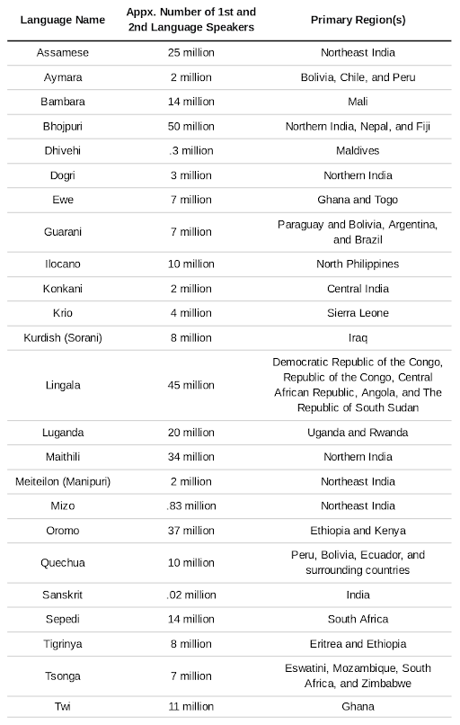Acknowledgements
We would like to first thank our coauthors – Yanping Huang, Ankur Bapna, Maxim Krikun, Dmitry Lepikhin and Minh-Thang Luong. We would also like to thank Wolfgang Macherey, Yuanzhong Xu, Zhifeng Chen and Macduff Richard Hughes for their helpful feedback. Special thanks to the Translate and Brain teams for their useful input and discussions, and the entire GShard development team for their foundational contributions to this project. We would also like to thank Tom Small for creating the animations for the blog post.