
 Efficient DGX System Sharing for Data Science Teams NVIDIA DGX is the universal system for AI and Data Science infrastructure. Hence, many organizations have incorporated DGX systems into their data centers for their data scientists and developers. The number of people running on these systems varies, from small teams of one to five people, to … Continued
Efficient DGX System Sharing for Data Science Teams
NVIDIA DGX is the universal system for AI and Data Science infrastructure. Hence, many organizations have incorporated DGX systems into their data centers for their data scientists and developers. The number of people running on these systems varies, from small teams of one to five people, to much larger teams of tens or maybe even hundreds of users. In this post we demonstrate how even a single DGX system can be efficiently utilized by multiple users. The focus in this blog is not on large DGX POD clusters. Rather, depending on the use cases, the deployment scale might be just one to several systems.
The deployment is managed via DeepOps toolkit, an open-source repository for common cluster management tasks. Using DeepOps organizations can customize features and scalability that are appropriate for their cluster and team sizes. Even when sharing just one DGX, users will have the capabilities and features of a rich cluster API to dynamically and efficiently run their workloads. That said, please note that DeepOps will require commitment from an organization’s DevOps professionals to tweak and maintain the underlying deployment. It is free and open-source software without support from NVIDIA.
DeepOps cluster API
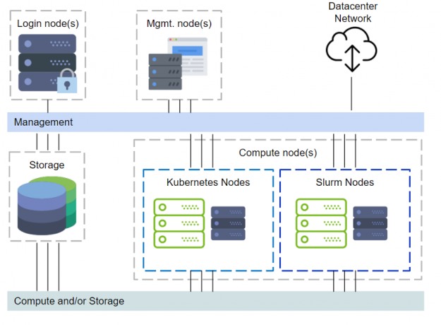
DeepOps covers setting up login nodes, management, monitoring, Kubernetes, Slurm, and even storage provisioning. Figure 1 illustrates a cluster with the DeepOps components.
The above setup with management nodes, Kubernetes and other components would require additional servers, either physical or virtual, to be provisioned. Some organizations might acquire just DGX systems, and even with one node this will be sufficient without additional servers to set up a multi-user environment. However, deploying Kubernetes with just one node is not supported. Refer to the “Zero to Data Science” blog on deploying Kubernetes. We will rely on Slurm for the cluster resource manager and scheduling. This limited scope is illustrated in Figure 2.
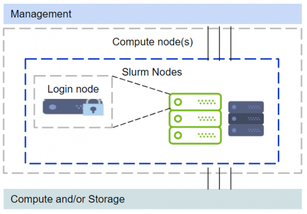
Since the major difference in this setup is that one of the compute nodes functions as a login node, a few modifications are recommended. The GPU devices are restricted from regular login ssh sessions. When a user needs to run something on a GPU they would need to start a Slurm job session. The requested GPUs would then be available within the Slurm job session.
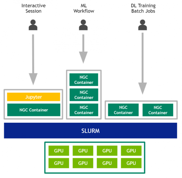
Additionally, in multi-user environments one typically wants to restrict elevated privileges for regular users. Rootless docker is used with the Slurm setup to avoid granting elevated rights to end users running containers. Rootless docker solves a couple problems. 1. The users can work in a familiar fashion with docker and NGC containers; 2. There is no need to add users to a privileged docker group; 3. The rootless docker sessions will be constrained to the Slurm job resources (privileged docker can bypass Slurm allocation constraints whereas rootless cannot).
In summary the users would interact with the GPUs per Figure 3.
DeepOps deployment instructions (single node options)
The DeepOps Slurm deployment instructions for single node setup are available on github.In this blog the platform is DGX. The recommended setup is the latest DGX OS with the latest firmware updates. A pristine freshly imaged DGX is preferred. Refer to the NVIDIA enterprise support portal for the latest DGX updates as well as the DGX release notes.
The steps shown in this document should be executed by a user with sudo privileges, such as the user created during initial DGX OS installation.
1. Clone the repo:
$ git clone https://github.com/NVIDIA/deepops.git
$ cd deepops
$ git checkout tags/21.06
2. Run initial setup script:
This will install Ansible and other prerequisite utilities for running deepops.
$ ./scripts/setup.sh
3. Edit config and options.
After running the setup script in step 2, a copy of “config.example” directory will be made to “config” directory. When one of the compute nodes also functions as a login node a few special configurations have to be set.
a. Configuring inventory “config/inventory”
Let a host be named “gpu01” (DGX-1 with 8 GPUs) with an ssh reachable ip address of “192.168.1.5” and some admin user “dgxuser”. Then a single node config would look like this:
$ vi config/inventory
[all]
gpu01     ansible_host=192.168.1.5

[slurm-master]
gpu01

[slurm-node]
gpu01

[all:vars]
# SSH User
ansible_user=dgxuser
ansible_ssh_private_key_file='~/.ssh/id_rsa'
If the machine has a different hostname (i.e. not gpu01), then use the desired host name. Running the deployment will change the hostname to what is set in the inventory file. Otherwise one can set the “deepops_set_hostname” var in “config/group_vars/all.yml” (refer to DeepOps Ansible configuration options).
Depending on how the ssh is configured on the cluster one might have to generate a passwordless private key. Leave the password blank when prompted:
$ ssh-keygen -t rsa
... accept defaults ...
$ cat ~/.ssh/id_rsa.pub >> ~/.ssh/authorized_keys
$ chmod 600 ./.ssh/authorized_keys
b. Configuring “config/group_vars/slurm-cluster.yml”
We need to add users to Slurm configuration for the ability to ssh as local users. This is needed when a compute node also functions as a login node. Additionally, set the singularity install option (which is “no” by default). Singularity can be used to run containers and it will be used to set up rootless options as well. Do not set up a default NFS with single node deployment.
$ vi config/group_vars/slurm-cluster.yml
slurm_allow_ssh_user:
- "user1"
- "user2"
- "user3”

slurm_login_on_compute: true

slurm_cluster_install_singularity: yes

slurm_enable_nfs_server: false
slurm_enable_nfs_client_nodes: false
Note: After deployment new users have to be manually added to “/etc/localusers” and “/etc/slurm/localusers.backup” on the node that functions as a login node.
4. Verify the configuration.
Check that ansible can run successfully and reach hosts. Run the hostname utility on “all” nodes. The “all” refers to the section in the “config/inventory” file. $ ansible all --connection=local -m raw -a "hostname"
For non-local setup does not set a connection to local. This requires ssh config to be set up properly in the “config/inventory”. Check connections via. $ ansible all -m raw -a "hostname"
5. Install Slurm.
When running Ansible, specify “–forks=1” so that Ansible does not perform potentially conflicting operations required for a slurm-master and slurm-node in parallel on the same node.The “–forks=1” option will ensure that the installation steps are serial.
$ ansible-playbook -K --forks=1 --connection=local -l slurm-cluster playbooks/slurm-cluster.ymlFor non-local installs do not set connection to local. The forks option is still required.
# NOTE: If SSH requires a password, add: `-k`
# NOTE: If sudo on remote machine requires a password, add: `-K`
# NOTE: If SSH user is different than current user, add: `-u ubuntu`
$ ansible-playbook -K --forks=1 -l slurm-cluster playbooks/slurm-cluster.yml
During Slurm playbook reboot is usually done twice:
- Once after installing the NVIDIA driver, because the driver sometimes requires a reboot to load correctly.
- Once after setting some grub options used for Slurm compute nodes to configure cgroups correctly, because of modification to the kernel command line.
The above reboot sequence cannot be automated when the compute and login nodes are on the same system. The recommended approach is to reboot manually when prompted and then run Ansible again. Setting “slurm_login_on_compute” to true, the slurm-cluster playbook will restrict GPUs in ssh sessions on the slurm-master by running the following command:
$ sudo systemctl set-property sshd.service DeviceAllow="/dev/nvidiactl"The reasoning for hiding GPUs in regular ssh sessions is that we want to avoid having users run a compute task on the GPUs without a Slurm job. If you desire to use docker within slurm then also install rootless docker after slurm deployment via playbook:
$ ansible-playbook -K --forks=1 --connection=local --limit slurm-cluster playbooks/container/docker-rootless.yml6. Post install information.
The admin users can access the GPUs that are restricted from regular ssh login sessions. This could be useful in situations when maybe GPU firmware needs to be updated. Let “dgxuser” be an admin user, they would access GPUs via command:
login-session:$ nvidia-smi -L
No devices found.
login-session:$ sudo systemd-run --scope --uid=root --gid=root -- bash
login-session-with-gpus:$ nvidia-smi -L | wc -l
8
Refer to official Slurm documentation for additional admin configurations and options. Typical Slurm options one might want to configure are time limits on jobs, accounts, qos and priority settings, etc.
Monitoring GPUs
Refer to DeepOps documentation regarding how monitoring is configured and deployed on the Slurm cluster.
The grafana dashboard will be available at the ip address of the manager node on port 3000 (with above config http://192.168.1.5:3000). Either open the url at the manager node’s ip address or tunnel. SSH tunnel example:
$ ssh -L localhost:3000:localhost:3000 dgxuser@192.168.1.5
# open url:
http://127.0.0.1:3000/
On RHEL the grafana service might need to be exposed via firewall-cmd.
$ firewall-cmd --zone=public --add-port=3000/tcp --permanent
$ firewall-cmd --reload
Logins and running jobs
After Slurm is deployed, the users can now request GPUs and run containers. The following examples demonstrate the working pattern for a multi-user team sharing a single DGX system.
Initial SSH to Login Node
Let the ip address of the login system be “192.168.1.5” and user “testuser”. They would ssh to the system as follows:
$ ssh testuser@192.168.1.5
testuser@192.168.1.5's password:
Welcome to NVIDIA DGX Server Version 5.0.0 (GNU/Linux 5.4.0-52-generic x86_64)

  System information as of Wed 09 Dec 2020 10:16:09 PM UTC

  System load:  0.11                Processes:                 908
  Usage of /:   12.9% of 437.02GB   Users logged in:           2
  Memory usage: 1%                  IPv4 address for docker0:  172.17.0.1
  Swap usage:   0%                  IPv4 address for enp1s0f0: 192.168.1.5
  Temperature:  47.0 C

The system has 0 critical alerts and 5 warnings. Use 'sudo nvsm show alerts' for more details.

Last login: Tue Dec  1 00:01:32 2020 from 172.20.176.144
login-session:$
At this point, the tester would not be able to run anything on GPUs. This is because the GPUs are not available to the user via the initial ssh login session.
login-session:$ nvidia-smi -L
No devices found.
It might be useful just in case to ssh again in another terminal window. The second login session could be used for monitoring jobs or to perform auxiliary tasks, whereas the first session would be used to launch jobs interactively (more on this in the following sections).
Allocating GPUs
To request a GPU the testuser must first run a Slurm command with GPU allocation. Example:
login-session:$ srun --ntasks=1 --cpus-per-task=5 --gpus-per-task=1 --pty bash
compute-session:$ nvidia-smi -L
GPU 0: Tesla P100-SXM2-16GB (UUID: GPU-61ba3c7e-584a-7eb4-d993-2d0b0a43b24f)
The job allocations details in Slurm can be viewed in another pane (such as one of the tmux panes in the login session without GPU access) via “squeue” command and details of the job can be viewed via “scontrol”.
             JOBID PARTITION     NAME     USER ST       TIME  NODES NODELIST(REASON)
               106     batch     bash testuser  R       3:34      1 gpu01
login-session:$ scontrol show jobid -dd 106
JobId=106 JobName=bash
UserId=testuser(1002) GroupId=testuser(1002) MCS_label=N/A
. . .
NumNodes=1 NumCPUs=6 NumTasks=1 CPUs/Task=5 ReqB:S:C:T=0:0:*:*
TRES=cpu=6,node=1,billing=6,gres/gpu=1
Socks/Node=* NtasksPerN:B:S:C=0:0:*:1 CoreSpec=*
JOB_GRES=gpu:1
Nodes=gpu01 CPU_IDs=0-5 Mem=0 GRES=gpu:1(IDX:0)
. . .DeepOps deploys Slurm with “pam_slurm_adopt” such that ssh sessions are permitted and adopted to allocated nodes. What that means is once a user has a Slurm job, additional ssh sessions will be adopted to the job. Proceeding with the above example, let us assume that job 106 is running. If the testuser were to make another ssh connection it would be adopted into job 106. If there were multiple jobs the default behaviour would be adopted into the latest job.
$ ssh testuser@192.168.1.5
testuser@192.168.1.5's password:
Welcome to NVIDIA DGX Server Version 5.0.0 (GNU/Linux 5.4.0-52-generic x86_64)
. . .
compute-session:$ echo NGPUS: $(nvidia-smi -L | wc -l) NCPUS: $(nproc)
NGPUS: 1 NCPUS: 6
Such ssh sessions are useful in various use cases: monitoring, debugging, additional launch commands, and so on. These adopted ssh sessions are automatically terminated when the corresponding Slurm job ends. The above scenario is also why it is convenient to use tmux with the initial ssh session.
Running containers
NVIDIA provides many AI, HPC, and Data Science containers. These are hosted on NGC. Take advantage of these GPU optimized containers. DeepOps enables running containers with several containerization alternatives: docker, singularity, and enroot with pyxis.
Rootless Docker
Docker remains the de facto industry standard for containerization. Docker is very easy to work with when building and extending containers. NGC and many other data science software stacks are distributed as docker containers. Fortunately, it is straightforward to incorporate rootless docker with Slurm. The reason for using rootless docker is that we want to avoid granting elevated privileges to users unnecessarily.
DeepOps sets up rootless docker as a module package. Environment modules are a popular way to set up cluster wide software for sharing. On a side note, DeepOps can set up easybuild or spack to manage environment modules and packages. The workflow with rootless docker is as follows: 1. A user starts a slurm job; 2. Module load the rootless docker package; 3. Start rootless docker daemon; 4. Work with docker containers per regular docker workflow. The following examples will illustrate the commands.
Start by reserving desired resources:
login-session:$ srun --ntasks=1 --gpus-per-task=4 --cpus-per-gpu=10
  --gpu-bind=closest --pty bash
Load and start rootless docker:
compute-session:$ module load rootless-docker
compute-session:$ start_rootless_docker.sh --quiet
The option “–quiet” redirects rootless docker messages to dev null to reduce verbosity. Then run a docker image:
compute-session:$ docker run --gpus=all --rm -it
  --shm-size=10g --ulimit memlock=-1 --ulimit stack=67108864
  nvcr.io/nvidia/tensorflow:21.04-tf2-py3
  mpirun --allow-run-as-root -H localhost:4
    --report-bindings --bind-to none --map-by slot -np 4
    python /workspace/nvidia-examples/cnn/resnet.py
The “–gpus=all” refers to all GPUs that are scheduled in the Slurm session, not all GPUs on the host. This could be placed in a script and run with srun or sbatch. Example:
$ cat test-resnetbench-docker.sh
#!/bin/bash

module load rootless-docker

start_rootless_docker.sh --quiet

docker run --gpus=all --rm -t
  --shm-size=10g --ulimit memlock=-1 --ulimit stack=67108864
  nvcr.io/nvidia/tensorflow:21.04-tf2-py3
  mpirun --allow-run-as-root -H localhost:4
    --report-bindings --bind-to none --map-by slot -np 4
    python /workspace/nvidia-examples/cnn/resnet.py

stop_rootless_docker.sh
Run the script:
login-session:$ srun --ntasks=1 --gpus-per-task=4 --cpus-per-gpu=10
  --gpu-bind=closest ${PWD}/test-resnetbench-docker.sh
The Slurm constraints are enforced for rootless docker. This can be verified by starting the container in an interactive slurm session and checking the number of GPUs and CPUs available.
login-session:$ srun --ntasks=1 --gpus-per-task=4 --cpus-per-gpu=10
  --gpu-bind=closest --pty bash
compute-session:$ module load rootless-docker
compute-session:$ start_rootless_docker.sh --quiet
compute-session:$ docker run --gpus=all --rm -it
  nvcr.io/nvidia/tensorflow:21.04-tf2-py3
  bash -c 'echo NGPUS: $(nvidia-smi -L | wc -l) NCPUS: $(nproc)'
NGPUS: 4 NCPUS: 40
Rootless docker runs via user namespace remapping. Files created are owned by the user, and within the container a user would not have write/execute permissions to filesystem or executables that the user already does not have permission to outside of the container. Thus user privileges are not elevated within Slurm when using rootless docker.
A user can explicitly stop the rootless docker daemon with “stop_rootless_docker.sh” script, or just exit the Slurm session. Upon ending a slurm session, processes in the session are killed and therefore the user’s rootless docker process will end.
compute-session:$ stop_rootless_docker.sh
compute-session:$ exit
exit
login-session:$
These scripts “start_rootless_docker.sh” and “stop_rootless_docker.sh” appear on a user’s path after loading the rootless docker module.
Enroot and singularity
Although beyond the scope of this blog, enroot and singularity could also be deployed via DeepOps. These are especially useful for multi-node jobs if running on more than one DGX system. The examples below though are for single node jobs.
Enroot with pyxis can be tested by running:
login-session:$ srun --mpi=pmi2 --ntasks=4 --gpus-per-task=1
  --cpus-per-gpu=10 --gpu-bind=closest
  --container-image='nvcr.io#nvidia/tensorflow:21.04-tf2-py3'
  python /workspace/nvidia-examples/cnn/resnet.py
The pyxis+enroot is invoked via option “–container-image” to run the container. Refer to enroot and pyxis documentation for further details.
Singularity could be used in a similar fashion to enroot. Using singularity it is typically more efficient to convert the docker container to singularity format (“*.sif”) prior to running the job. Don’t forget the “–nv” option for GPUs. Example:
login-session:$ singularity pull docker://nvcr.io/nvidia/tensorflow:21.04-tf2-py3
login-session:$ srun --mpi=pmi2 --ntasks=4 --gpus-per-task=1
  --cpus-per-gpu=10 --gpu-bind=closest
  singularity exec --nv ~/singularity_images/tensorflow_21.04-tf2-py3.sif
  python /workspace/nvidia-examples/cnn/resnet.py
Refer to singularity documentation for further details. Building containers with singularity is permitted to non-privileged users via the “–fakeroot” option.
Enroot and Singularity excel at running containerized multinode jobs, which is somewhat difficult and less convenient to do using docker on Slurm. The focus of the blog is on single node DeepOps deployment, but if multinode containerized jobs on Slurm are of interest consider enroot and singularity for that task.
Conclusion
DeepOps aims to make managing GPU clusters flexible and scalable. Various organizations ranging from enterprises to small businesses, startups, and educational institutions, can adopt and deploy DeepOps features relevant to their teams. Admins have tools at their disposal to manage GPUs effectively. Meanwhile, users can collaborate and work productively and efficiently on shared GPU resources.
Get started with DeepOps and refer to the tips in this blog to work productively with your GPUs and DGX systems.
- Link to DeepOps: DeepOps
- Landing Product Page: DGX Systems
- Solutions Page: Data Center
- Newsletter: Data Science Newsletter


 NVIDIA Omniverse has expanded to address the scientific visualization community with aConnector to Kitware ParaView, one of the world’s most popular scientific visualization applications.