
 Robotics researchers from NVIDIA and University of Southern California recently presented their work at the 2021 RSS conference called DiSECt, the first differentiable simulator for robotic cutting.
Robotics researchers from NVIDIA and University of Southern California presented their work at the 2021 Robotics: Science and Systems (RSS) conference called DiSECt, the first differentiable simulator for robotic cutting. The simulator accurately predicts the forces acting on a knife as it presses and slices through natural soft materials, such as fruits and vegetables.
Robots that are intelligent, adaptive and generalize cutting behavior with either a kitchen butter knife, or a surgical resection remains a difficult problem for researchers.
As it turns out, the process of cutting with feedback requires adaptation to stiffness of the objects, applied force during the cut, and often a sawing motion to cut through. To achieve this, researchers use a family of techniques which leverage feedback to guide the controller adaptation. However, fluid controller adaptation requires very careful parameter tuning for each instance of the same problem. While these techniques are successful in industrial settings, no two cucumbers (or tomatoes) are the same, hence rendering these family of algorithms ineffective in a more generic setting.
In contrast, recent focus in research has been in building differentiable algorithms for control problems, which in simpler terms means that the sensitivity of output with respect to input can be evaluated without excessive sampling. Efficient solutions for control problems are achievable when the simulated dynamics is differentiable [1,2,3], but the process of simulating cutting has not been differentiable so far!
Differentiable simulation for cutting poses a challenge, since naturally cutting is a discontinuous process where crack formation and fracture propagation occur that prohibit the calculation of gradients. We tackle this problem by proposing a novel way of simulating cutting that represents the process of crack propagation and damage mechanics in a continuous manner.
DiSECt implements the commonly used Finite Element Method (FEM) to simulate deformable materials, such as foodstuffs. The object to be cut is represented by a 3D mesh which consists of tetrahedral elements. Along the cutting surface we slice the mesh following the Virtual Node Algorithm [4]. This algorithm duplicates the mesh elements that intersect the cutting surface, and adds additional, so-called “virtual” vertices on the edges where these elements are cut. The virtual nodes add extra degrees of freedom to accurately simulate the contact dynamics of the knife when it presses and slices through the mesh.
Next, DiSECt inserts springs connecting the virtual nodes on either side of the cutting surface. These cutting springs allow us to simulate damage mechanics and crack propagation in a continuous manner, by weakening them in proportion to the contact force the knife exerts on the mesh. This continuous treatment allows us to differentiate through the dynamics in order to compute gradients for the parameters defining the properties of the material or the trajectory of the knife. For example, given the gradients for the vertical and sideways velocity of the knife, we can efficiently determine an energy-minimizing yet fast cutting motion through gradient-based optimization.

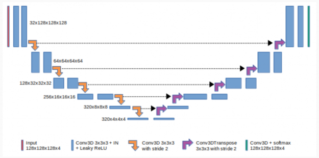
We leverage reverse-mode automatic differentiation to efficiently compute gradients for hundreds of simulation parameters. Our simulator uses source code transformation which automatically generates efficient CUDA kernels for the forward and backward passes of all our simulation routines, such as the FEM or contact model. Such an approach allows us to implement complex simulation routines which are parallelized on the GPU, while the gradients of the inputs with respect to the outputs of such routines are automatically derived from analyzing the abstract syntax tree (AST) of the simulation code.
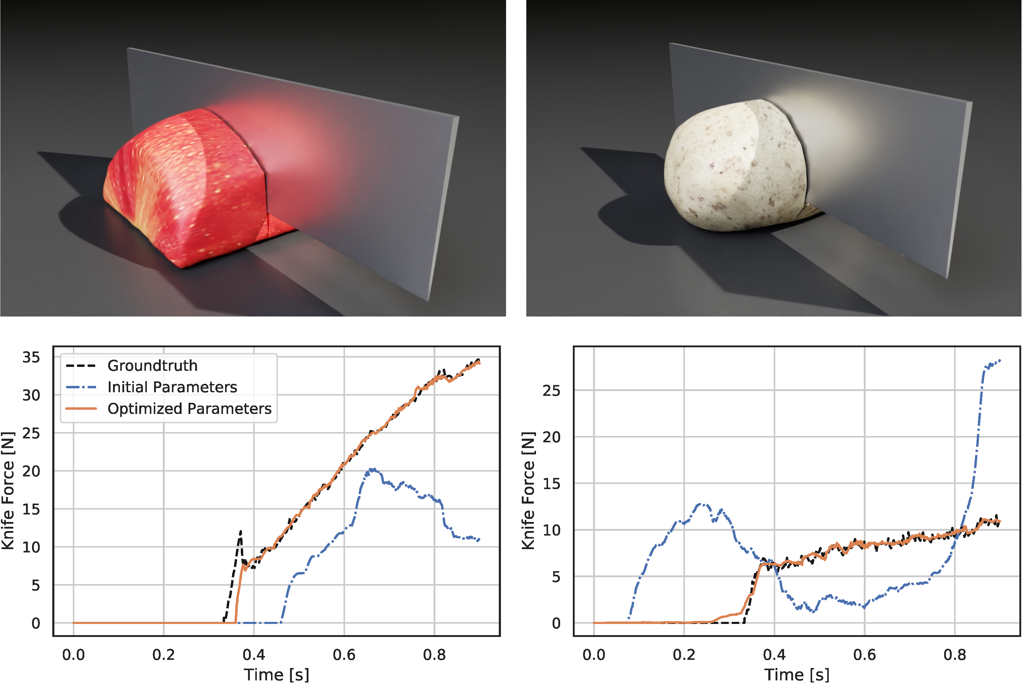
Through gradient-based optimization algorithms, we can automatically tune the simulation parameters to achieve a close match between the simulator and real-world measurements. In one of our experiments, we leverage an existing dataset [5] of knife force profiles measured by a real-world robot while cutting various foodstuffs. We set up our simulator with the corresponding mesh and its material properties, and optimize the remaining parameters to reduce the discrepancy between the simulated and the real knife force profile. Within 150 gradient evaluations, our simulator closely predicts the knife force profile, as we demonstrate on the examples of cutting an actual apple and a potato. As shown in the figure, the initial parameter guess yielded a force profile that was far from the real observation, and our approach automatically found an accurate fit. We present further results in our accompanying paper that demonstrate that the found parameters generalize to different conditions, such as the downward velocity of the knife or the length of the reference trajectory window.
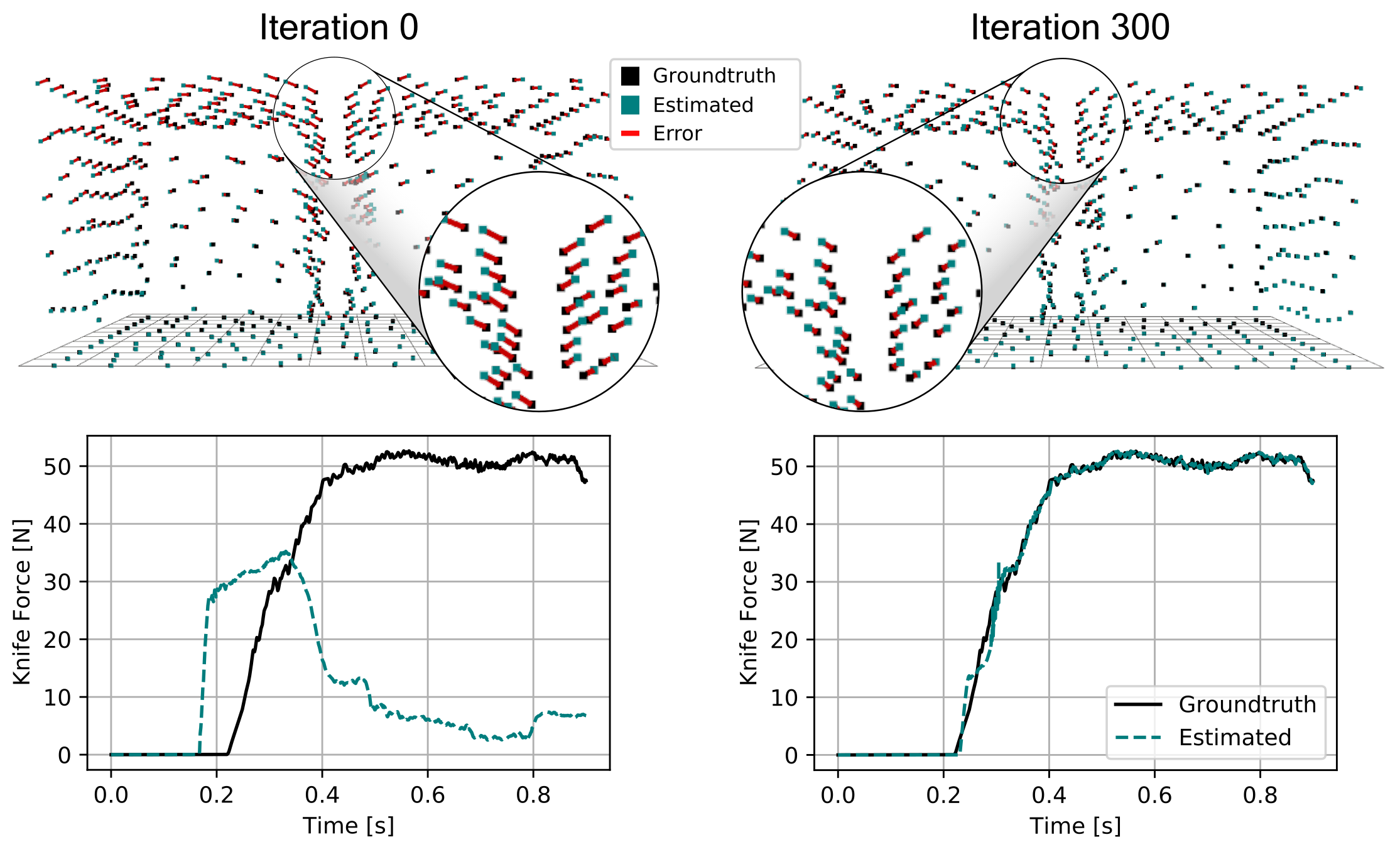
We also generate additional data using a highly established commercial simulator, which allows us to precisely control the experimental setup, such as object shape and material properties. Given such data, we can also leverage the motion of the mesh vertices as an additional ground-truth signal. After optimizing the simulation parameters, DiSECt is able to predict the vertex positions and velocities, as well as the force profile, much more accurately.
Aside from parameter inference, the gradients of our differentiable cutting simulator can also be used to optimize the cutting motion of the knife. In our full cutting simulation, we represent a trajectory by keyframes, where each frame prescribes the downward velocity, as well as the frequency and amplitude of a sinusoidal sideways velocity. At the start of the optimization, the initial motion is a straight downward-pressing motion.
We optimize this trajectory with the objective to minimize the mean force on the knife and penalize the time it takes to cut the object. Studies have shown that humans perform sawing motions when cutting biomaterials in order to reduce the required force. Such behavior emerges from our optimization as well.
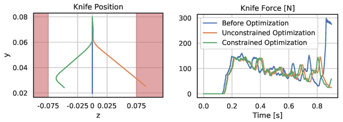
After 50 iterations with the Adam optimizer, we see a reduction in average knife force by 15 percent. However, the knife slices sideways further than its blade length. Therefore, we add a hard constraint to keep the lateral motion within valid limits and perform constrained optimization. Thanks to the end-to-end-differentiability of DiSECt, accurate gradients for such constraints are available, and lead to a valid knife motion which requires only 0.3 percent more force than the unconstrained result.
Cutting food items multiple times results in slightly different force profiles for each instance, depending on the geometry of such materials. We additionally present results to transfer simulation parameters between different meshes corresponding to the same material. Our approach leverages optimal transport to find correspondences between simulation parameters of a source mesh and a target mesh (e.g., local stiffnesses) based on the location of the virtual nodes. As shown in the following figure, the 2D positions of these nodes along the cutting surface allow us to map simulation parameters (shown here is the softness of the cutting springs) to topologically different target geometries.
In our ongoing research, we are bringing our differentiable simulation approach to real-world robotic cutting. We investigate a closed-loop control system where the simulator is updated online from force measurements, while the robot is cutting foodstuffs. Through model-predictive planning and optimal control, we aim to find time- and energy-efficient cutting actions that apply to the physical system.
We thank Yan-Bin Jia and Prajjwal Jamdagni for kindly providing us a dataset of real-world cutting trajectories which we used throughout our experiments. Be sure to also check out their research on robotic cutting!
DiSECt is a finalist at 2021 RSS for the best (student) paper. Visit the team’s project webpage to learn more.
DiSECt Research Paper: DiSECt: A Differentiable Simulation Engine for Autonomous Robotic Cutting
Eric Heiden, Miles Macklin, Yashraj S Narang, Dieter Fox, Animesh Garg, Fabio Ramos
Robotics Science and Systems (RSS) 2021.


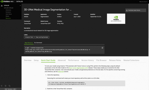
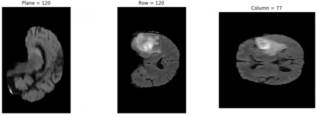
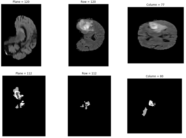
 The NVIDIA NGC team is hosting a webinar with live Q&A to dive into this Jupyter notebook available from the NGC catalog. Learn how to use these resources to kickstart your AI journey. Register now: NVIDIA NGC Jupyter Notebook Day: Medical Imaging Segmentation. Image segmentation partitions a digital image into multiple segments by changing the …
 ![NGC catalog page shows cards for GPU-optimized HPC and AI containers, pretrained models, and industry SDKs that help accelerate workflows]](https://developer-blogs.nvidia.com/wp-content/uploads/2021/07/NGC-catalog-625x381.png)
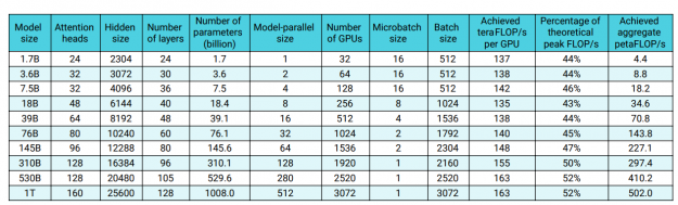
") Despite unprecedented progress in NLP, many state-of-the-art models are available in English only. NVIDIA has developed tools to enable the development of even the largest language models. This post describes the challenges associated with building and deploying large scale models and the solutions to enable global organizations to achieve NLP leadership in their regions.
Despite unprecedented progress in NLP, many state-of-the-art models are available in English only. NVIDIA has developed tools to enable the development of even the largest language models. This post describes the challenges associated with building and deploying large scale models and the solutions to enable global organizations to achieve NLP leadership in their regions.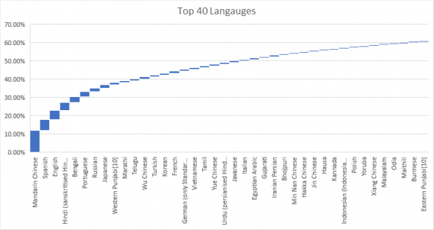

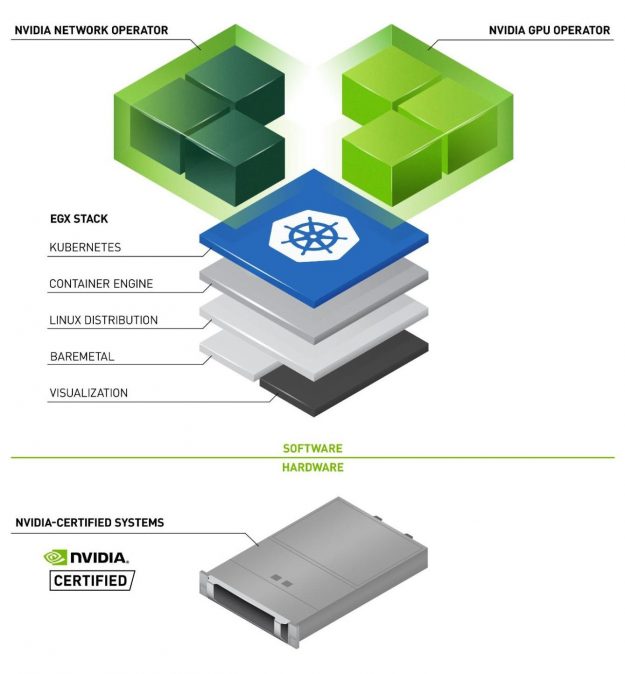
 NVIDIA EGX contains the NVIDIA GPU Operator and the new NVIDIA Network Operator 1.0 to standardize and automate the deployment of all the necessary components for provisioning Kubernetes clusters. Now released for use in production environments, the NVIDIA Network Operator makes Kubernetes networking simple and effortless for bringing AI to the enterprise.
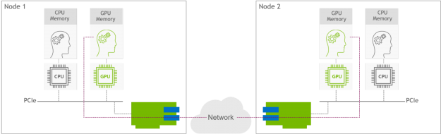
 The NVIDIA Hardware Grant Program helps advance AI and data science by partnering with academic institutions around the world to enable researchers and educators with industry-leading hardware and software.