GeForce NOW gives you the power to game almost anywhere, at GeForce quality. And with the latest controller from SteelSeries, members can stay in control of the action on Android and Chromebook devices. This GFN Thursday takes a look at the SteelSeries Stratus+, now part of the GeForce NOW Recommended program. And it wouldn’t be Read article >
From the documentation and forum discussions, I learnt that these embeddings are the output of a pretrained model (MFCC+CNN) of the 10 second chunks of respective youtube videos. I have also learnt that these embeddings make it easy to work on deep learning models. How does it help the ML engineers?
My confusion is if these audio embeddings are already pre-trained, what are the utilities of these audio embeddings? i.e. How can I use these embeddings to train advanced models for performing Sound Event Detection?
Hello! So I am trying to create a multiclass classifier using VGG16 in transfer learning to classify users’I emotions. The data is sorted into 4 classes, which have their proper directories so I can use the ‘image_dataset_from_directory’ function.
My code correctly identifies X number of images to 4 classes, but when I try to execute model.fit() it returns this error:
ValueError: in user code: File "/home/blabs/.local/lib/python3.9/site-packages/keras/engine/training.py", line 878, in train_function * return step_function(self, iterator) File "/home/blabs/.local/lib/python3.9/site-packages/keras/engine/training.py", line 867, in step_function ** outputs = model.distribute_strategy.run(run_step, args=(data,)) File "/home/blabs/.local/lib/python3.9/site-packages/keras/engine/training.py", line 860, in run_step ** outputs = model.train_step(data) File "/home/blabs/.local/lib/python3.9/site-packages/keras/engine/training.py", line 809, in train_step loss = self.compiled_loss( File "/home/blabs/.local/lib/python3.9/site-packages/keras/engine/compile_utils.py", line 201, in __call__ loss_value = loss_obj(y_t, y_p, sample_weight=sw) File "/home/blabs/.local/lib/python3.9/site-packages/keras/losses.py", line 141, in __call__ losses = call_fn(y_true, y_pred) File "/home/blabs/.local/lib/python3.9/site-packages/keras/losses.py", line 245, in call ** return ag_fn(y_true, y_pred, **self._fn_kwargs) File "/home/blabs/.local/lib/python3.9/site-packages/keras/losses.py", line 1664, in categorical_crossentropy return backend.categorical_crossentropy( File "/home/blabs/.local/lib/python3.9/site-packages/keras/backend.py", line 4994, in categorical_crossentropy target.shape.assert_is_compatible_with(output.shape) ValueError: Shapes (None, 1) and (None, 4) are incompatible
How can I approach solving this issue? Thank you for your help.
We have a Tensorflow workflow and model that works great when used in a local environment (Python) – however, we now need to push it to production (Heroku). So we’re thinking we need to move our model into some type of Cloud hosting.
If possible, I’d like to upload the model directory (not an H5 file) to a cloud service/storage provider and then load that model into Tensorflow.
Here is how we’re currently loading in a model, and what we’d like to be able to do:
# Current setup loads model from local directory dnn_model = tf.keras.models.load_model('./neural_network/true_overall) # We'd like to be able to load the model from a cloud service/storage dnn_model = tf.keras.models.load_model('https://some-kinda-storage-service.com/neural_network/true_overall)
Downloading the directory and running it from a temp directory isn’t an option with our setup – so we’ll need to be able to run the model from the cloud. We don’t necessarily need to “train” the model in the cloud, we just need to be able to load it.
I’ve looked into some things like TensorServe and TensorCloud, but I’m not 100% sure if thats what we need (we’re super new to Tensorflow and AI in general).
What’s the best way to get the models (as a directory) into the cloud so we can load them into our code?
Posted by Mohammad Saleh, Software Engineer, Google Research, Brain Team and Anjuli Kannan, Software Engineer, Google Docs
For many of us, it can be challenging to keep up with the volume of documents that arrive in our inboxes every day: reports, reviews, briefs, policies and the list goes on. When a new document is received, readers often wish it included a brief summary of the main points in order to effectively prioritize it. However, composing a document summary can be cognitively challenging and time-consuming, especially when a document writer is starting from scratch.
To help with this, we recently announced that Google Docs now automatically generates suggestions to aid document writers in creating content summaries, when they are available. Today we describe how this was enabled using a machine learning (ML) model that comprehends document text and, when confident, generates a 1-2 sentence natural language description of the document content. However, the document writer maintains full control — accepting the suggestion as-is, making necessary edits to better capture the document summary or ignoring the suggestion altogether. Readers can also use this section, along with the outline, to understand and navigate the document at a high level. While all users can add summaries, auto-generated suggestions are currently only available to Google Workspace business customers. Building on grammar suggestions, Smart Compose, and autocorrect, we see this as another valuable step toward improving written communication in the workplace.
A blue summary icon appears in the top left corner when a document summary suggestion is available. Document writers can then view, edit, or ignore the suggested document summary.
Abstractive text summarization, which combines the individually challenging tasks of long document language understanding and generation, has been a long-standing problem in NLU and NLG research. A popular method for combining NLU and NLG is training an ML model using sequence-to-sequence learning, where the inputs are the document words, and the outputs are the summary words. A neural network then learns to map input tokens to output tokens. Early applications of the sequence-to-sequence paradigm used recurrent neural networks (RNNs) for both the encoder and decoder.
The introduction of Transformers provided a promising alternative to RNNs because Transformers use self-attention to provide better modeling of long input and output dependencies, which is critical in document summarization. Still, these models require large amounts of manually labeled data to train sufficiently, so the advent of Transformers alone was not enough to significantly advance the state-of-the-art in document summarization.
The combination of Transformers with self-supervised pre-training (e.g., BERT, GPT, T5) led to a major breakthrough in many NLU tasks for which limited labeled data is available. In self-supervised pre-training, a model uses large amounts of unlabeled text to learn general language understanding and generation capabilities. Then, in a subsequent fine-tuning stage, the model learns to apply these abilities on a specific task, such as summarization or question answering.
The Pegasus work took this idea one step further, by introducing a pre-training objective customized to abstractive summarization. In Pegasus pre-training, also called Gap Sentence Prediction (GSP), full sentences from unlabeled news articles and web documents are masked from the input and the model is required to reconstruct them, conditioned on the remaining unmasked sentences. In particular, GSP attempts to mask sentences that are considered essential to the document through different heuristics. The intuition is to make the pre-training as close as possible to the summarization task. Pegasus achieved state-of-the-art results on a varied set of summarization datasets. However, a number of challenges remained to apply this research advancement into a product.
Applying Recent Research Advances to Google Docs
Data
Self-supervised pre-training results in an ML model that has general language understanding and generation capabilities, but a subsequent fine-tuning stage is critical for the model to adapt to the application domain. We fine-tuned early versions of our model on a corpus of documents with manually-generated summaries that were consistent with typical use cases.
However, early versions of this corpus suffered from inconsistencies and high variation because they included many types of documents, as well as many ways to write a summary — e.g., academic abstracts are typically long and detailed, while executive summaries are brief and punchy. This led to a model that was easily confused because it had been trained on so many different types of documents and summaries that it struggled to learn the relationships between any of them.
Fortunately, one of the key findings in the Pegasus work was that an effective pre-training phase required less supervised data in the fine-tuning stage. Some summarization benchmarks required as few as 1,000 fine-tuning examples for Pegasus to match the performance of Transformer baselines that saw 10,000+ supervised examples — suggesting that one could focus on quality rather than quantity.
We carefully cleaned and filtered the fine-tuning data to contain training examples that were more consistent and represented a coherent definition of summaries. Despite the fact that we reduced the amount of training data, this led to a higher quality model. The key lesson, consistent with recent work in domains like dataset distillation, was that it was better to have a smaller, high quality dataset, than a larger, high-variance dataset.
Serving
Once we trained the high quality model, we turned to the challenge of serving the model in production. While the Transformer version of the encoder-decoder architecture is the dominant approach to train models for sequence-to-sequence tasks like abstractive summarization, it can be inefficient and impractical to serve in real-world applications. The main inefficiency comes from the Transformer decoder where we generate the output summary token by token through autoregressive decoding. The decoding process becomes noticeably slow when summaries get longer since the decoder attends to all previously generated tokens at each step. RNNs are a more efficient architecture for decoding since there is no self-attention with previous tokens as in a Transformer model.
We used knowledge distillation, which is the process of transferring knowledge from a large model to a smaller more efficient model, to distill the Pegasus model into a hybrid architecture of a Transformer encoder and an RNN decoder. To improve efficiency we also reduced the number of RNN decoder layers. The resulting model had significant improvements in latency and memory footprint while the quality was still on par with the original model. To further improve the latency and user experience, we serve the summarization model using TPUs, which provide significant speed ups and allow more requests to be handled by a single machine.
Ongoing Challenges and Next Steps While we are excited by the progress so far, there are a few challenges we are continuing to tackle:
Document coverage: Developing a set of documents for the fine-tuning stage was difficult due to the tremendous variety that exists among documents, and the same challenge is true at inference time. Some of the documents our users create (e.g., meeting notes, recipes, lesson plans and resumes) are not suitable for summarization or can be difficult to summarize. Currently, our model only suggests a summary for documents where it is most confident, but we hope to continue broadening this set as our model improves.
Evaluation: Abstractive summaries need to capture the essence of a document while being fluent and grammatically correct. A specific document may have many summaries that can be considered correct, and different readers may prefer different ones. This makes it hard to evaluate summaries with automatic metrics only, user feedback and usage statistics will be critical for us to understand and keep improving quality.
Long documents: Long documents are some of the toughest documents for the model to summarize because it is harder to capture all the points and abstract them in a single summary, and it can also significantly increase memory usage during training and serving. However, long documents are perhaps most useful for the model to automatically summarize because it can help document writers get a head start on this tedious task. We hope we can apply the latest ML advancements to better address this challenge.
Conclusion Overall, we are thrilled that we can apply recent progress in NLU and NLG to continue assisting users with reading and writing. We hope the automatic suggestions now offered in Google Workspace make it easier for writers to annotate their documents with summaries, and help readers comprehend and navigate documents more easily.
Acknowledgements The authors would like to thank the many people across Google that contributed to this work: AJ Motika, Matt Pearson-Beck, Mia Chen, Mahdis Mahdieh, Halit Erdogan, Benjamin Lee, Ali Abdelhadi, Michelle Danoff, Vishnu Sivaji, Sneha Keshav, Aliya Baptista, Karishma Damani, DJ Lick, Yao Zhao, Peter Liu, Aurko Roy, Yonghui Wu, Shubhi Sareen, Andrew Dai, Mekhola Mukherjee, Yinan Wang, Mike Colagrosso, and Behnoosh Hariri. .
Turn on your TV. Fire up your favorite streaming service. Grab a Coke. A demo of the most important visual technology of our time is as close as your living room couch. Propelled by an explosion in computing power over the past decade and a half, path tracing has swept through visual media. It brings Read article >
I would like to share my project and show you how to apply tinyML approach to detect broken tooth conditions in the gearbox based upon recorded vibration data.
I used Raspberry Pi Pico, Arduino IDE, Neuton Tiny ML software I will give an answer to such a questions as:
Is it possible to make an AI-driven system that predicts gearbox failure on a simple $4 MCU? How to automatically build a compact model that does not require any additional compression? Can a non-data scientist implement such projects successfully?
Introduction and Business Constraint
In industry (e.g., wind power, automotive), gearboxes often operate under random speed variations. A condition monitoring system is expected to detect faults, broken tooth conditions and assess their severity using vibration signals collected under different speed profiles.
Modern cars have hundreds of thousands of details and systems where it is necessary to predict breakdowns, control the state of temperature, pressure, etc.As such, in the automotive industry, it is critically important to create and embed TinyML models that can perform right on the sensors and open up a set of technological advantages, such as:
Internet independence
No waste of energy and money on data transfer
Advanced privacy and security
In my experiment I want to show how to easily create such a technology prototype to popularize the TinyML approach and use its incredible capabilities for the automotive industry.
Neuton TinyML:Neuton**,** I selected this solution since it is free to use and automatically creates tiny machine learning models deployable even on 8-bit MCUs. According to Neuton developers, you can create a compact model in one iteration without compression.
Raspberry Pi Pico: The chip employs two ARM Cortex-M0 + cores, 133 megahertz, which are also paired with 256 kilobytes of RAM when mounted on the chip. The device supports up to 16 megabytes of off-chip flash storage, has a DMA controller, and includes two UARTs and two SPIs, as well as two I2C and one USB 1.1 controller. The device received 16 PWM channels and 30 GPIO needles, four of which are suitable for analog data input. And with a net $4 price tag.
The goal of this tutorial is to demonstrate how you can easily build a compact ML model to solve a multi-class classification task to detect broken tooth conditions in the gearbox.
Dataset Description
Gearbox Fault Diagnosis Dataset includes the vibration dataset recorded by using SpectraQuest’s Gearbox Fault Diagnostics Simulator.
Dataset has been recorded using 4 vibration sensors placed in four different directions and under variation of load from ‘0’ to ’90’ percent. Two different scenarios are included:1) Healthy condition 2) Broken tooth condition
There are 20 files in total, 10 for a healthy gearbox and 10 for a broken one. Each file corresponds to a given load from 0% to 90% in steps of 10%. You can find this dataset through the link: https://www.kaggle.com/datasets/brjapon/gearbox-fault-diagnosis
The experiment will be conducted on a $4 MCU, with no cloud computing carbon footprints 🙂
Step 1: Model training
For model training, I’ll use the free of charge platform, Neuton TinyML. Once the solution is created, proceed to the dataset uploading (keep in mind that the currently supported format is CSV only).
Number of coefficients = 397, File Size for Embedding = 2.52 Kb. That’s super cool! It is a really small model!Upon the model training completion, click on the Prediction tab, and then click on the Download button next to Model for Embedding to download the model library file that we are going to use for our device.
Step 2: Embedding on Raspberry Pico
Once you have downloaded the model files, it’s time to add our custom functions and actions. I am using Arduino IDE to program Raspberry Pico.
Note: Since we are going to make classification on the test dataset, we will use the CSV utility provided by Neuton to run inference on the data sent to the MCU via USB.
I tried to build the same model with TensorFlow and TensorFlow Lite as well. My model built with Neuton TinyML turned out to be 4.3% better in terms of Accuracy and 15.3 times smaller in terms of model size than the one built with TF Lite. Speaking of the number of coefficients, TensorFlow’s model has, 9, 330 coefficients, while Neuton’s model has only 397 coefficients (which is 23.5 times smaller than TF!).
The resultant model footprint and inference time are as follows:
Autonomous vehicle development and validation require the ability to replicate real-world scenarios in simulation. At GTC, NVIDIA founder and CEO Jensen Huang showcased new AI-based tools for NVIDIA DRIVE Sim that accurately reconstruct and modify actual driving scenarios. These tools are enabled by breakthroughs from NVIDIA Research that leverage technologies such as NVIDIA Omniverse platform Read article >
This week at GTC, we’re celebrating – celebrating the amazing and impactful work that developers and startups are doing around the world. Nowhere is that more apparent than among the members of our global NVIDIA Inception program, designed to nurture cutting-edge startups who are revolutionizing industries. The program is free for startups of all sizes Read article >
Warp is a Python API framework for writing GPU graphics and simulation code, especially within Omniverse.
Typically, real-time physics simulation code is written in low-level CUDA C++ for maximum performance. In this post, we introduce NVIDIA Warp, a new Python framework that makes it easy to write differentiable graphics and simulation GPU code in Python. Warp provides the building blocks needed to write high-performance simulation code, but with the productivity of working in an interpreted language like Python.
By the end of this post, you learn how to use Warp to author CUDA kernels in your Python environment and make use of some of the built-in high-level functionality that makes it easy to write complex physics simulations, such as an ocean simulation (Figure 1).
Figure 1. Ocean simulation in Omniverse using Warp
Installation
Warp is available as an open-source library from GitHub. When the repository has been cloned, you can install it using your local package manager. For pip, use the following command:
pip install warp
Initialization
After importing, you must explicitly initialize Warp:
import warp as wp
wp.init()
Launching kernels
Warp uses the concept of Python decorators to mark functions that can be executed on the GPU. For example, you could write a simple semi-implicit particle integration scheme as follows:
Because Warp is strongly typed, you should provide type hints to kernel arguments. To launch a kernel, use the following syntax:
    wp.launch(kernel=simple_kernel, # kernel to launch
              dim=1024,             # number of threads
              inputs=[a, b, c],     # parameters
              device="cuda")        # execution device
Unlike tensor-based frameworks such as NumPy, Warp uses a kernel-based programming model. Kernel-based programming more closely matches the underlying GPU execution model. It is often a more natural way to express simulation code that requires fine-grained conditional logic and memory operations. However, Warp exposes this thread-centric model of programming in an easy-to-use way that does not require low-level knowledge of GPU architecture.
Compilation model
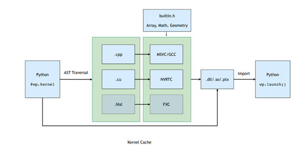
Launching a kernel triggers a just-in-time (JIT) compilation pipeline that automatically generates C++/CUDA kernel code from Python function definitions.
All kernels belonging to a Python module are runtime compiled into dynamic libraries and PTX. Figure 2. shows the compilation pipeline, which involves traversing the function AST and converting this to straight-line CUDA code that is then compiled and loaded back into the Python process.
Figure 2. Compilation pipeline for Warp kernels
The result of this JIT compilation is cached. If the input kernel source is unchanged, then the precompiled binaries are loaded in a low-overhead fashion.
Memory model
Memory allocations in Warp are exposed through the warp.array type. Arrays wrap an underlying memory allocation that may live in either host (CPU), or device (GPU) memory. Unlike tensor frameworks, arrays in Warp are strongly typed and store a linear sequence of built-in structures (vec3, matrix33, quat, and so on).
You can construct arrays from Python lists or NumPy arrays, or initialized, using a similar syntax to NumPy and PyTorch:
# allocate an uninitizalized array of vec3s
    v = wp.empty(length=n, dtype=wp.vec3, device="cuda")

    # allocate a zero-initialized array of quaternions
    q = wp.zeros(length=n, dtype=wp.quat, device="cuda")

    # allocate and initialize an array from a numpy array
    # will be automatically transferred to the specified device
    v = wp.from_numpy(array, dtype=wp.vec3, device="cuda")
Warp supports the __array_interface__, and __cuda_array_interface__ protocols, which allow zero-copy data views between tensor-based frameworks. For example, to convert data to NumPy use the following command:
# automatically bring data from device back to host
    view = device_array.numpy()
Features
Warp includes several higher-level data structures that make implementing simulation and geometry processing algorithms easier.
Meshes
Triangle meshes are ubiquitous in simulation and computer graphics. Warp provides a built-in type for managing mesh data that provide support for geometric queries, such as closest point, ray-cast, and overlap checks.
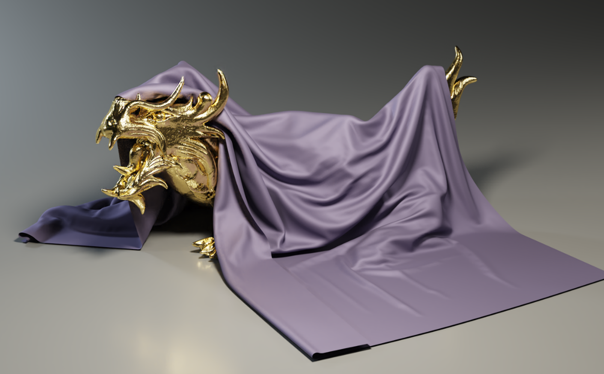
The following example shows how to use Warp to compute the closest point on a mesh to an array of input positions. This type of computation is the building block for many algorithms in collision detection (Figure 3). Warp’s mesh queries make it simple to implement such methods.
Figure 3. An example of collision detection against a complex object that uses closest-point mesh queries to test for contact between particles and the underlying object
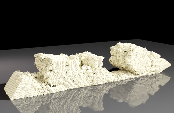
Sparse volumes are incredibly useful for representing grid data over large domains, such as signed distance fields (SDFs) for complex objects or velocities for large-scale fluid flow. Warp includes support for sparse volumes defined using the NanoVDB standard. Construct volumes using standard OpenVDB tools such as Blender, Houdini, or Maya, and then sample inside Warp kernels.
You can create volumes directly from binary grid files on disk or in-memory, and then sample them using the volumes API:
wp.volume_sample_world(vol, xyz, mode)  # world space sample using interpolation mode
wp.volume_sample_local(vol, uvw, mode)  # volume space sample using interpolation mode
wp.volume_lookup(vol, ijk)              # direct voxel lookup
wp.volume_transform(vol, xyz)           # map point from voxel space to world space
wp.volume_transform_inv(vol, xyz)       # map point from world space to volume space
Figure 4. A particle simulation where the rock formation is represented as a sparse NanoVDB level set
Using volume queries, you can efficiently collide against complex objects with minimal memory overhead.
Hash grids
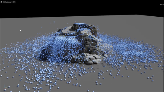
Many particle-based simulation methods, such as the discrete element method (DEM) or smoothed particle hydrodynamics (SPH), involve iterating over spatial neighbors to compute force interactions. Hash grids are a well-established data structure to accelerate these nearest neighbor queries and are particularly well suited to the GPU.
Hash grids are constructed from point sets as follows:
When hash grids are created, you can query them directly from within user kernel code as shown in the following example, which computes the sum of all neighbor particle positions:
@wp.kernel
def sum(grid : wp.uint64,
points: wp.array(dtype=wp.vec3),
output: wp.array(dtype=wp.vec3),
radius: float):
tid = wp.tid()
# query point
p = points[tid]
# create grid query around point
query = wp.hash_grid_query(grid, p, radius)
index = int(0)
sum = wp.vec3()
while(wp.hash_grid_query_next(query, index)):
neighbor = points[index]
# compute distance to neighbor point
dist = wp.length(p-neighbor)
if (dist
Figure 5 shows an example of a DEM granular material simulation for a cohesive material. Using the built-in hash-grid data structure allows you to write such a simulation in fewer than 200 lines of Python and runs at interactive rates for more than 100K particles.
Figure 5. An example of a DEM granular material simulation
Using the Warp hash-grid data allows you to easily evaluate the pairwise force interactions between neighboring particles.
Differentiability
Tensor-based frameworks, such as PyTorch and JAX, provide gradients of tensor computations and are well-suited for applications like ML training.
A unique feature of Warp is the ability to generate forward and backward versions of kernel code. This makes it easy to write differentiable simulations that can propagate gradients as part of a larger training pipeline. A common scenario is to use traditional ML frameworks for network layers, and Warp to implement simulation layers allowing for end-to-end differentiability.
When gradients are required, you should create arrays with requires_grad=True. For example, the warp.Tape class can record kernel launches and replay them to compute the gradient of a scalar loss function with respect to the kernel inputs:
After the backward pass has completed, the gradients with respect to the inputs are available through a mapping in the Tape object:
# gradient of loss with respect to input a
print(tape.gradients[a])
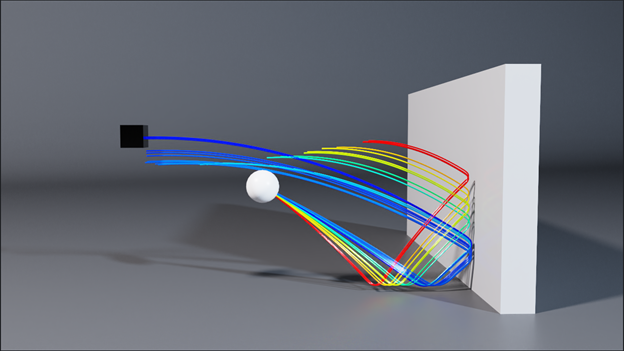
Figure 6. A trajectory optimization example where the initial velocity of the ball is optimized to hit the black target. Each line shows the result of one iteration of an LBFGS optimization step.
Summary
In this post, we presented NVIDIA Warp, a Python framework that makes it easy to write differentiable simulation code for the GPU. We encourage you to download the Warp preview release, share results, and give us feedback.
For more information, see the following resources:


 Warp is a Python API framework for writing GPU graphics and simulation code, especially within Omniverse.
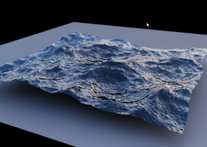