cuSOLVERMp provides a distributed-memory multi-node and multi-GPU solution for solving systems of linear equations at scale! In the future, it will also solve eigenvalue and singular value problems.
Today, cuSOLVERMp version 0.0.1 is now available at no charge for members of the NVIDIA Developer Program.
The Early Access release targets P9 + IBM’s Spectrum MPI
About cuSOLVERMp
cuSOLVERMp provides a distributed-memory multi-node and multi-GPU solution for solving systems of linear equations at scale! In the future, it will also solve eigenvalue and singular value problems.
Future releases will be hosted in the HPC SDK. It will provide additional functionality and support for x86_64 + OpenMPI.
Posted by Nachiappan Valliappan, Senior Software Engineer and Kai Kohlhoff, Staff Research Scientist, Google Research
Eye movement has been studied widely across vision science, language, and usability since the 1970s. Beyond basic research, a better understanding of eye movement could be useful in a wide variety of applications, ranging across usability and user experience research, gaming, driving, and gaze-based interaction for accessibility to healthcare. However, progress has been limited because most prior research has focused on specialized hardware-based eye trackers that are expensive and do not easily scale.
In “Accelerating eye movement research via accurate and affordable smartphone eye tracking”, published in Nature Communications, and “Digital biomarker of mental fatigue”, published in npj Digital Medicine, we present accurate, smartphone-based, ML-powered eye tracking that has the potential to unlock new research into applications across the fields of vision, accessibility, healthcare, and wellness, while additionally providing orders-of-magnitude scaling across diverse populations in the world, all using the front-facing camera on a smartphone. We also discuss the potential use of this technology as a digital biomarker of mental fatigue, which can be useful for improved wellness.
Model Overview The core of our gaze model was a multilayer feed-forward convolutional neural network (ConvNet) trained on the MIT GazeCapture dataset. A face detection algorithm selected the face region with associated eye corner landmarks, which were used to crop the images down to the eye region alone. These cropped frames were fed through two identical ConvNet towers with shared weights. Each convolutional layer was followed by an average pooling layer. Eye corner landmarks were combined with the output of the two towers through fully connected layers. Rectified Linear Units (ReLUs) were used for all layers except the final fully connected output layer (FC6), which had no activation.
Architecture of the unpersonalized gaze model. Eye regions, extracted from a front-facing camera image, serve as input into a convolutional neural network. Fully-connected (FC) layers combine the output with eye corner landmarks to infer gaze x– and y-locations on screen via a multi-regression output layer.
The unpersonalized gaze model accuracy was improved by fine-tuning and per-participant personalization. For the latter, a lightweight regression model was fitted to the model’s penultimate ReLU layer and participant-specific data.
Model Evaluation To evaluate the model, we collected data from consenting study participants as they viewed dots that appeared at random locations on a blank screen. The model error was computed as the distance (in cm) between the stimulus location and model prediction. Results show that while the unpersonalized model has high error, personalization with ~30s of calibration data led to an over fourfold error reduction (from 1.92 to 0.46cm). At a viewing distance of 25-40 cm, this corresponds to 0.6-1° accuracy, a significant improvement over the 2.4-3° reported in previous work [1, 2].
Additional experiments show that the smartphone eye tracker model’s accuracy is comparable to state-of-the-art wearable eye trackers both when the phone is placed on a device stand, as well as when users hold the phone freely in their hand in a near frontal headpose. In contrast to specialized eye tracking hardware with multiple infrared cameras close to each eye, running our gaze model using a smartphone’s single front-facing RGB camera is significantly more cost effective (~100x cheaper) and scalable.
Using this smartphone technology, we were able to replicate key findings from prior eye movement research in neuroscience and psychology, including standard oculomotor tasks (to understand basic visual functioning in the brain) and natural image understanding. For example, in a simple prosaccade task, which tests a person’s ability to quickly move their eyes towards a stimulus that appears on the screen, we found that the average saccade latency (time to move the eyes) matches prior work for basic visual health (210ms versus 200-250ms). In controlled visual search tasks, we were able to replicate key findings, such as the effect of target saliency and clutter on eye movements.
Example gaze scanpaths show the effect of the target’s saliency (i.e., color contrast) on visual search performance. Fewer fixations are required to find a target (left) with high saliency (different from the distractors), while more fixations are required to find a target (right) with low saliency (similar to the distractors).
For complex stimuli, such as natural images, we found that the gaze distribution (computed by aggregating gaze positions across all participants) from our smartphone eye tracker are similar to those obtained from bulky, expensive eye trackers that used highly controlled settings, such as laboratory chin rest systems. While the smartphone-based gaze heatmaps have a broader distribution (i.e., they appear more “blurred”) than hardware-based eye trackers, they are highly correlated both at the pixel level (r = 0.74) and object level (r = 0.90). These results suggest that this technology could be used to scale gaze analysis for complex stimuli such as natural and medical images (e.g., radiologists viewing MRI/PET scans).
Similar gaze distribution from our smartphone approach vs. a more expensive (100x) eye tracker (from the OSIE dataset).
We found that smartphone gaze could also help detect difficulty with reading comprehension. Participants reading passages spent significantly more time looking within the relevant excerpts when they answered correctly. However, as comprehension difficulty increased, they spent more time looking at the irrelevant excerpts in the passage before finding the relevant excerpt that contained the answer. The fraction of gaze time spent on the relevant excerpt was a good predictor of comprehension, and strongly negatively correlated with comprehension difficulty (r = −0.72).
Digital Biomarker of Mental Fatigue Gaze detection is an important tool to detect alertness and wellbeing, and is studied widely in medicine, sleep research, and mission-critical settings such as medical surgeries, aviation safety, etc. However, existing fatigue tests are subjective and often time-consuming. In our recent paper published in npj Digital Medicine, we demonstrated that smartphone gaze is significantly impaired with mental fatigue, and can be used to track the onset and progression of fatigue.
A simple model predicts mental fatigue reliably using just a few minutes of gaze data from participants performing a task. We validated these findings in two different experiments — using a language-independent object-tracking task and a language-dependent proofreading task. As shown below, in the object-tracking task, participants’ gaze initially follows the object’s circular trajectory, but under fatigue, their gaze shows high errors and deviations. Given the pervasiveness of phones, these results suggest that smartphone-based gaze could provide a scalable, digital biomarker of mental fatigue.
Example gaze scanpaths for a participant with no fatigue (left) versus with mental fatigue (right) as they track an object following a circular trajectory.
The corresponding progression of fatigue scores (ground truth) and model prediction as a function of time on task.
Beyond wellness, smartphone gaze could also provide a digital phenotype for screening or monitoring health conditions such as autism spectrum disorder, dyslexia, concussion and more. This could enable timely and early interventions, especially for countries with limited access to healthcare services.
Another area that could benefit tremendously is accessibility. People with conditions such as ALS, locked-in syndrome and stroke have impaired speech and motor ability. Smartphone gaze could provide a powerful way to make daily tasks easier by using gaze for interaction, as recently demonstrated with Look to Speak.
Ethical Considerations Gaze research needs careful consideration, including being mindful of the correct use of such technology — applications should obtain explicit approval and fully informed consent from users for the specific task at hand. In our work, all data was collected for research purposes with users’ explicit approval and consent. In addition, users were allowed to opt out at any point and request their data to be deleted. We continue to research additional ways to ensure ML fairness and improve the accuracy and robustness of gaze technology across demographics, in a responsible, privacy-preserving way.
Conclusion Our findings of accurate and affordable ML-powered smartphone eye tracking offer the potential for orders-of-magnitude scaling of eye movement research across disciplines (e.g., neuroscience, psychology and human-computer interaction). They unlock potential new applications for societal good, such as gaze-based interaction for accessibility, and smartphone-based screening and monitoring tools for wellness and healthcare.
Acknowledgements This work involved collaborative efforts from a multidisciplinary team of software engineers, researchers, and cross-functional contributors. We’d like to thank all the co-authors of the papers, including our team members, Junfeng He, Na Dai, Pingmei Xu, Venky Ramachandran; interns, Ethan Steinberg, Kantwon Rogers, Li Guo, and Vincent Tseng; collaborators, Tanzeem Choudhury; and UXRs: Mina Shojaeizadeh, Preeti Talwai, and Ran Tao. We’d also like to thank Tomer Shekel, Gaurav Nemade, and Reena Lee for their contributions to this project, and Vidhya Navalpakkam for her technical leadership in initiating and overseeing this body of work.
Background Predictive maintenance is used for early fault detection, diagnosis, and prediction when maintenance is needed in various industries including oil and gas, manufacturing, and transportation. Equipment is continuously monitored to measure things like sound, vibration, and temperature to alert and report potential issues. To accomplish this in computers, the first step is to determine … Continued
Background
Predictive maintenance is used for early fault detection, diagnosis, and prediction when maintenance is needed in various industries including oil and gas, manufacturing, and transportation. Equipment is continuously monitored to measure things like sound, vibration, and temperature to alert and report potential issues. To accomplish this in computers, the first step is to determine the root cause of any type of failure or error. The current industry-standard practice uses complex rulesets to continuously monitor specific components, but such systems typically only alert on previously observed faults. In addition, these regular expressions (regex) rulesets do not scale. As data becomes more voluminous and heterogeneous, maintaining these rulesets presents a neverending catch-up task. Since they only alert on what has been seen in the past, they cannot detect new root causes with patterns that were unknown to analysts before.
The approach
To create a more proactive approach for predictive maintenance, we’ve implemented uses Natural Language Processing (NLP) to monitor and interpret kernel logs. The RAPIDS CLX team collaborated with the NVIDIA Enterprise Experience (NVEX) team to test and run a proof-of-concept (POC) to evaluate this NLP-based solution. The project seeks to:
Drastically reduce the time spent manually analyzing kernel logs of NVIDIA DGX systems by pinpointing important lines in the vast amount of logs,
Probabilistically classify sequences, giving the team the capability to fine-tune a threshold to decide whether a line in the log is a root cause or not.
Figure 1: Workflow using NVIDIA DGX Systems for Log Parsing in and Predictive Maintenance Use Case.
A complete example of a root cause workflow can be found in the RAPIDS CLX GitHub repository. For final deployment past the POC, the team is using NVIDIA Morpheus, an open AI framework for developers to implement cybersecurity-specific inference pipelines. Morpheus provides a simple interface for security developers and data scientists to create and deploy end-to-end pipelines that address cybersecurity, information security, and general log-based pipelines. It is built on a number of other pieces of technology, including RAPIDS, Triton, TensorRT, Streamz, CLX, and more.
The POC is outlined as follows:
The first step identifies root causes that caused past failures. NVEX provides a dataset that contains lines in kernel logs that have been marked as a root cause to date.
Next, the problem is framed as a classification problem by sorting the logs into two groups, ordinary, and root cause. Ordinary logs are labeled as 0 and root cause lines as 1.
We have fine-tuned a pre-trained BERT model from HuggingFace to perform classification. More information about the BERT model can be found in the original paper. The code block below shows the pre-trained model called “bert-base-uncased” is loaded to be used for sequence classification.
Like validation accuracy, test set accuracy is also close to one, which means most of the predicted classes are the same as the original labels. We performed an inference run for classification with two goals:
Check the number of false positives. In our context, this means the number of lines in the kernel logs that are predicted to be a root cause but are not of interest.
Check the number of false negatives. In our context, this refers to the lines that are root causes but predicted to be ordinary.
Unlike the conventional evaluation of classification tasks, having a labelled test set does not translate into interpretable results as one of our main targets is to predict previously unseen root causes. The best way to understand how the model performs is to check the resulting confusion matrix.
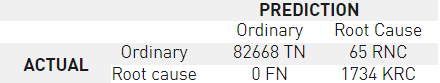
Table 1: Confusion matrix for root cause analysis prediction
In our use case, the confusion matrix gives the following outputs:
TN (True Negatives): These are the ordinary lines that were not labeled as a root cause, and the model correctly marks 82668 of them.
FN (False Negatives): Zero false negatives mean the model does not mark any of the known root causes as ordinary.
NRC (New Root Causes): 65 new lines that were marked as ordinary are predicted to be root causes. These are the lines that would have been missed with the existing methods.
KRC (Known Root Causes): This is the number of lines correctly marked as root cause.
NVEX analysts have reviewed our predictions and noticed some interesting logs that were not marked as a root cause of issues with the conventional methods. With regex-based methods, such new issues might have cost a significant amount of person-hours to triage, develop, and harden.
Applying our solution to more use cases
In the next phase, we plan to position similar solutions in NVIDIA platforms to alert users of potential problems or execute corrective actions with Morpheus. By building on the success of root cause analysis here, we seek to extend this into a predictive maintenance task by continuous monitoring of the logs. This use case is certainly not limited to DGX systems. For example, telecommunication infrastructure equipment, including radio, core, and transmission devices, generate a diverse set of logs. Their outages may result in loss of service and severe fines. Identifying the root cause of outages imposes a significant cost, both in terms of dollars spent and person-hours. We believe all systems that generate text-based logs, especially the ones that run mission-critical applications, would benefit from such NLP based predictive maintenance solutions immensely as it would reduce the mean time to resolution.
Recently, at GTC21, the NVIDIA CloudXR team ran a Connect with Experts session about the CloudXR SDK. We shared how CloudXR can deliver limitless virtual and augmented reality over networks (including 5G) to low cost, low-powered headsets and devices, all while maintaining the high-quality experience traditionally reserved for high-end headsets that are plugged into high-performance … Continued
Recently, at GTC21, the NVIDIA CloudXR team ran a Connect with Experts session about the CloudXR SDK. We shared how CloudXR can deliver limitless virtual and augmented reality over networks (including 5G) to low cost, low-powered headsets and devices, all while maintaining the high-quality experience traditionally reserved for high-end headsets that are plugged into high-performance computers.
Q&A session
At the end of this session, we hosted a Q&A with our panel of professional visualization solution architects and received a large number of questions from our audience. VR and AR director David Weinstein and senior manager Greg Jones from the NVIDIA CloudXR team provided answers to the top questions:
How are you addressing instances of running XR with large crowds such as convention centers or large public places?
The number of users at a single physical location is gated by the wireless spectrum capacity at that given location.
Do you need separate apps on both the client and the server?
The CloudXR SDK provides sample CloudXR clients (including source code) for a variety of client devices. The server side of CloudXR gets installed as a SteamVR plug-in and can stream all OpenVR applications.
Can I use CloudXR if I do not have high-end hardware?
CloudXR will run with a variety of hardware. For the server side, all VR-Ready GPUs from the Pascal and later architectures are supported. For the client side, CloudXR has been tested with HTC Vive, HTC Vive Pro, HTC Focus Plus, Oculus Quest, Oculus Quest 2, Valve Index, and HoloLens2.
Can the server be shared for multiple simultaneous clients or is this one server per one client only?
Currently, we only support one server per one client device. In a virtualized environment this means one virtual machine per one client.
Is connectivity (server to network to client) bidirectional?
Yes, the connectivity is bidirectional. The pose information and controller input data is streamed from the client to the server; frames, audio and haptics are streamed from the server to the client.
Figure 1. CloudXR configurations
What type of applications run with NVIDIA CloudXR?
OpenVR applications run with CloudXR.
More information
To learn more, visit the CloudXR page where there are plenty of videos, blog posts, webinars, and more to help you get started. Did you miss GTC21? The AR/VR sessions are available for free through NVIDIA On-Demand.
Introduction Modern natural language processing (NLP) mixes modeling, feature engineering, and general text processing. Deep learning NLP models can provide fantastic performance for tasks like named-entity recognition (NER), sentiment classification, and text summarization. However, end-to-end workflow pipelines with these models often struggle with a performance at scale, especially when the pipelines involve extensive pre-and post-inference … Continued
This post was originally published on the RAPIDS AI Blog.
TLDR: Learn how to use RAPIDS, HuggingFace, and Dask for high-performance NLP. See how to build end-to-end NLP pipelines in a fast and scalable way on GPUs. This covers feature engineering, deep learning inference, and post-inference processing.
Introduction
Modern natural language processing (NLP) mixes modeling, feature engineering, and general text processing. Deep learning NLP models can provide fantastic performance for tasks like named-entity recognition (NER), sentiment classification, and text summarization. However, end-to-end workflow pipelines with these models often struggle with a performance at scale, especially when the pipelines involve extensive pre-and post-inference processing.
In our previous blog post, we covered how RAPIDS accelerates string processing and feature engineering. This post explains how to leverage RAPIDS for feature engineering and string processing, HuggingFace for deep learning inference, and Dask for scaling out for end-to-end acceleration on GPUs.
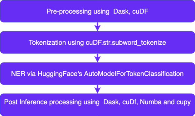
An NLP pipeline often involves the following steps:
Pre-processing
Tokenization
Inference
Post Inference Processing
Figure 1: NLP workflow using Rapids and HuggingFace.
Pre-Processing:
Pre-Processing for NLP pipelines involves general data ingestion, filtration, and general reformatting. With the RAPIDS ecosystem, each piece of the workflow is accelerated on GPUs. Check out our recent blog where we showcased these capabilities in more detail.
Once we have pre-processed our data, we need to tokenize it so that the appropriate machine learning model can ingest it.
Subword Tokenization:
Tokenization is the process of breaking down the text into standard units that a machine can understand. It is a fundamental step across NLP methods from traditional like CountVectorizer to advanced deep learning methods like Transformers.
One approach to tokenization is breaking a sentence into words. For example, the sentence, “I love apples” can be broken down into, “I,” “love,” “apples”. But this delimiter based tokenization runs into problems like:
Needing a large vocabulary as you will need to store all words in the dictionary.
Uncertainty of combined words like “check-in,” i.e., what exactly constitutes a word, is often ambiguous.
Some languages don’t segment by spaces.
To solve these problems, we use subword tokenization. Subword tokenization is a recent strategy from machine translation that breaks into subword units, strings of characters like “ing,” “any,” “place.” For example, the word “anyplace” can be broken down into “any” and “place,” so you don’t need an entry for each word in your vocabulary.
When BERT(Bidirectional Encoder Representations from Transformers) was released in 2018, it included a new subword algorithm called WordPiece. This tokenization is used to create input for NLP DL models like BERT, Electra, DistilBert, and more.
GPU Subword Tokenization
We first introduced the GPU BERT subword tokenizer in a previous blog as part of CLX for cybersecurity applications. Since then, we migrated the implementation into RAPIDS cuDF and exposed it as a string function, subword tokenization, making it easier to use in typical DataFrame workflows.
This tokenizer takes a series of strings and returns tokenized cupy arrays:
Tokens are extracted and kept in GPU memory and then used in subsequent tensors, all without leaving GPUs and avoiding expensive CPU copies.
Once our inputs are tokenized using the subword tokenizer, they can be fed into NLP DL models like BERT for inference.
HuggingFace Overview:
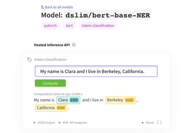
HuggingFace provides access to several pre-trained transformer model architectures ( BERT, GPT-2, RoBERTa, XLM, DistilBert, XLNet…) for Natural Language Understanding (NLU) and Natural Language Generation (NLG) with over 32+ pre-trained models in 100+ languages.In our workflow, we used BERT and DISTIILBERT from HuggingFace to do named entity recognition.
This section covers how we put RAPIDS, HuggingFace, and Dask together to achieve 5x better performance than theleading Apache Spark and OpenNLP for TPCx-BB query 27 equivalent pipeline at the 10TB scale factor with 136 V100 GPUs while using a near state of the art NER model. We expect to see even better results with A100 as A100’s BERT inference speed is up to 6x faster than V100’s.
In this workflow, we are given 26 Million synthetic reviews, and the task is to find the competitor company names in the product reviews for a given product. We then return the review id, product id, competitor company name, and the related sentence from the online review. To get a competitor’s name, we need to do NER on the reviews and find all the tokens in the review labeled as an organization.
Our previous implementation relied on spaCy for NER but, spaCy currently needs your inputs on CPU and thus was slow as it required a copy to CPU memory and back to GPU memory. With the new cudf.str.subword_tokenize, we can go from cudf.string.series to subword tensors without leaving the GPU unlocking many new SOTA language models.
In this task, we experimented with two of HuggingFace’s models for NER fine-tuned on CoNLL 2003(English) :
Bert-base-model: This model gets an f1 of 91.95and achieves a speedup of 1.7 x over spaCy.
Research by Zhu, Mengdi et al. (2019) showcased that BERT-based model architectures achieve near state art performance, significantly improving the performance on existing public-NER toolkits like spaCy, NLTK, and StanfordNER.
For example, the bert-basemodel on average across datasets achieves a 13.63% better F1 than spaCy, so not only did we get faster but also reached near state of the art performance.
This workflow is just one example of leveraging GPUs to do end to end accelerating natural language processing. With cudf.str.subword_tokenizenow, most of the NLP tasks such as question answering, text-classification, summarization, translation, token classification are all within reach for an end to end acceleration leveraging RAPIDS and HuggingFace.Stay tuned for more examples and in, the meantime, try out RAPIDS in your NLP work on Google Colab or blazingsql notebooks, see our documentation docs page, and if you see something missing, we welcome feature requests on GitHub!
Hello, I had an older tensorflow model written in V1 of tensorflow. It has been quite a while, and I have forgotten how the model works, and how to print the summary of the model in tensorflow v1. What is the syntax to print the summary, I tried model.summary() but it returns an error.
These are the lines that the program runs to initiate training.
for i in range(epochs):traind_scores = []ii = 0epoch_loss = []while(ii + batch_size) <= len(X_train):X_batch = X_train[ii:ii+batch_size]y_batch = y_train[ii:ii+batch_size]
o, c, _ = session.run([outputs, loss, trained_optimizer], feed_dict={inputs:X_batch, targets:y_batch})
epoch_loss.append(c)traind_scores.append(o)ii += batch_sizeprint(‘Epoch {}/{}’.format(i, epochs), ‘ Current loss: {}’.format(np.mean(epoch_loss)))
How can I change the parameter based on my input model? I have 4 input to predict 1 output. In one example I saw I have 1 input that predicts 1 output and the scale parameter is set to 1?
Posted by Zarana Parekh, Software Engineer and Jason Baldridge, Staff Research Scientist, Google Research
The past decade has seen remarkable progress on automatic image captioning, a task in which a computer algorithm creates written descriptions for images. Much of the progress has come through the use of modern deep learning methods developed for both computer vision and natural language processing, combined with large scale datasets that pair images with descriptions created by people. In addition to supporting important practical applications, such as providing descriptions of images for visually impaired people, these datasets also enable investigations into important and exciting research questions about grounding language in visual inputs. For example, learning deep representations for a word like “car”, means using both linguistic and visual contexts.
Image captioning datasets that contain pairs of textual descriptions and their corresponding images, such as MS-COCO and Flickr30k, have been widely used to learn aligned image and text representations and to build captioning models. Unfortunately, these datasets have limited cross-modal associations: images are not paired with other images, captions are only paired with other captions of the same image (also called co-captions), there are image-caption pairs that match but are not labeled as a match, and there are no labels that indicate when an image-caption pair does not match. This undermines research into how inter-modality learning (connecting captions to images, for example) impacts intra-modality tasks (connecting captions to captions or images to images). This is important to address, especially because a fair amount of work on learning from images paired with text is motivated by arguments about how visual elements should inform and improve representations of language.
To address this evaluation gap, we present “Crisscrossed Captions: Extended Intramodal and Intermodal Semantic Similarity Judgments for MS-COCO“, which was recently presented at EACL 2021. The Crisscrossed Captions (CxC) dataset extends the development and test splits of MS-COCO with semantic similarity ratings for image-text, text-text and image-image pairs. The rating criteria are based on Semantic Textual Similarity, an existing and widely-adopted measure of semantic relatedness between pairs of short texts, which we extend to include judgments about images as well. In all, CxC contains human-derived semantic similarity ratings for 267,095 pairs (derived from 1,335,475 independent judgments), a massive extension in scale and detail to the 50k original binary pairings in MS-COCO’s development and test splits. We have released CxC’s ratings, along with code to merge CxC with existing MS-COCO data. Anyone familiar with MS-COCO can thus easily enhance their experiments with CxC.
Crisscrossed Captions extends the MS-COCO evaluation sets by adding human-derived semantic similarity ratings for existing image-caption pairs and co-captions (solid lines), and it increases rating density by adding human ratings for new image-caption, caption-caption and image-image pairs (dashed lines).*
Creating the CxC Dataset If a picture is worth a thousand words, it is likely because there are so many details and relationships between objects that are generally depicted in pictures. We can describe the texture of the fur on a dog, name the logo on the frisbee it is chasing, mention the expression on the face of the person who has just thrown the frisbee, or note the vibrant red on a large leaf in a tree above the person’s head, and so on.
The CxC dataset extends the MS-COCO evaluation splits with graded similarity associations within and across modalities. MS-COCO has five captions for each image, split into 410k training, 25k development, and 25k test captions (for 82k, 5k, 5k images, respectively). An ideal extension would rate every pair in the dataset (caption-caption, image-image, and image-caption), but this is infeasible as it would require obtaining human ratings for billions of pairs.
Given that randomly selected pairs of images and captions are likely to be dissimilar, we came up with a way to select items for human rating that would include at least some new pairs with high expected similarity. To reduce the dependence of the chosen pairs on the models used to find them, we introduce an indirect sampling scheme (depicted below) where we encode images and captions using different encoding methods and compute the similarity between pairs of same modality items, resulting in similarity matrices. Images are encoded using Graph-RISE embeddings, while captions are encoded using two methods — Universal Sentence Encoder (USE) and average bag-of-words (BoW) based on GloVe embeddings. Since each MS-COCO example has five co-captions, we average the co-caption encodings to create a single representation per example, ensuring all caption pairs can be mapped to image pairs (more below on how we select intermodality pairs).
Top: Text similarity matrix (each cell corresponds to a similarity score) constructed using averaged co-caption encodings, so each text entry corresponds to a single image, resulting in a 5k x 5k matrix. Two different text encoding methods were used, but only one text similarity matrix has been shown for simplicity. Bottom: Image similarity matrix for each image in the dataset, resulting in a 5k x 5k matrix.
The next step of the indirect sampling scheme is to use the computed similarities of images for a biased sampling of caption pairs for human rating (and vice versa). For example, we select two captions with high computed similarities from the text similarity matrix, then take each of their images, resulting in a new pair of images that are different in appearance but similar in what they depict based on their descriptions. For example, the captions “A dog looking bashfully to the side” and “A black dog lifts its head to the side to enjoy a breeze” would have a reasonably high model similarity, so the corresponding images of the two dogs in the figure below could be selected for image similarity rating. This step can also start with two images with high computed similarities to yield a new pair of captions. We now have indirectly sampled new intramodal pairs — at least some of which are highly similar — for which we obtain human ratings.
Top: Pairs of images are picked based on their computed caption similarity. Bottom: Pairs of captions are picked based on the computed similarity of the images they describe.
Last, we then use these new intramodal pairs and their human ratings to select new intermodal pairs for human rating. We do this by using existing image-caption pairs to link between modalities. For example, if a caption pair example ij was rated by humans as highly similar, we pick the image from example i and caption from example j to obtain a new intermodal pair for human rating. And again, we use the intramodal pairs with the highest rated similarity for sampling because this includes at least some new pairs with high similarity. Finally, we also add human ratings for all existing intermodal pairs and a large sample of co-captions.
The following table shows examples of semantic image similarity (SIS) and semantic image-text similarity (SITS) pairs corresponding to each rating, with 5 being the most similar and 0 being completely dissimilar.
Examples for each human-derived similarity score (left: 5 to 0, 5 being very similar and 0 being completely dissimilar) of image pairs based on SIS (middle) and SITS (right) tasks. Note that these examples are for illustrative purposes and are not themselves in the CxC dataset.
Evaluation MS-COCO supports three retrieval tasks:
Given an image, find its matching captions out of all other captions in the evaluation set.
Given a caption, find its corresponding image out of all other images in the evaluation set.
Given a caption, find its other co-captions out of all other captions in the evaluation set.
MS-COCO’s pairs are incomplete because captions created for one image at times apply equally well to another, yet these associations are not captured in the dataset. CxC enhances these existing retrieval tasks with new positive pairs, and it also supports a new image-image retrieval task. With its graded similarity judgements, CxC also makes it possible to measure correlations between model and human rankings. Retrieval metrics in general focus only on positive pairs, while CxC’s correlation scores additionally account for the relative ordering of similarity and include low-scoring items (non-matches). Supporting these evaluations on a common set of images and captions makes them more valuable for understanding inter-modal learning compared to disjoint sets of caption-image, caption-caption, and image-image associations.
We ran a series of experiments to show the utility of CxC’s ratings. For this, we constructed three dual encoder (DE) models using BERT-base as the text encoder and EfficientNet-B4 as the image encoder:
A text-text (DE_T2T) model that uses a shared text encoder for both sides.
An image-text model (DE_I2T) that uses the aforementioned text and image encoders, and includes a layer above the text encoder to match the image encoder output.
A multitask model (DE_I2T+T2T) trained on a weighted combination of text-text and image-text tasks.
CxC retrieval results — a comparison of our text-text (T2T), image-text (I2T) and multitask (I2T+T2T) dual encoder models on all the four retrieval tasks.
From the results on the retrieval tasks, we can see that DE_I2T+T2T (yellow bar) performs better than DE_I2T (red bar) on the image-text and text-image retrieval tasks. Thus, adding the intramodal (text-text) training task helped improve the intermodal (image-text, text-image) performance. As for the other two intramodal tasks (text-text and image-image), DE_I2T+T2T shows strong, balanced performance on both of them.
CxC correlation results for the same models shown above.
For the correlation tasks, DE_I2T performs the best on SIS and DE_I2T+T2T is the best overall. The correlation scores also show that DE_I2T performs well only on images: it has the highest SIS but has much worse STS. Adding the text-text loss to DE_I2T training (DE_I2T+T2T) produces more balanced overall performance.
The CxC dataset provides a much more complete set of relationships between and among images and captions than the raw MS-COCO image-caption pairs. The new ratings have been released and further details are in our paper. We hope to encourage the research community to push the state of the art on the tasks introduced by CxC with better models for jointly learning inter- and intra-modal representations.
Acknowledgments The core team includes Daniel Cer, Yinfei Yang and Austin Waters. We thank Julia Hockenmaier for her inputs on CxC’s formulation, the Google Data Compute Team, especially Ashwin Kakarla and Mohd Majeed for their tooling and annotation support, Yuan Zhang, Eugene Ie for their comments on the initial versions of the paper and Daphne Luong for executive support for the data collection.
* All the images in the article have been taken from the Open Images dataset under the CC-by 4.0 license.
Recommender systems (RecSys) have become a key component in many online services, such as e-commerce, social media, news service, or online video streaming. However with the growth in importance, the growth in scale of industry datasets, and more sophisticated models, the bar has been raised for computational resources required for recommendation systems. To meet the … Continued
Recommender systems (RecSys) have become a key component in many online services, such as e-commerce, social media, news service, or online video streaming. However with the growth in importance, the growth in scale of industry datasets, and more sophisticated models, the bar has been raised for computational resources required for recommendation systems.
To meet the computational demands for large-scale DL recommender systems, NVIDIA introduced Merlin – a Framework for Deep Recommender Systems. Now NVIDIA teams have won two consecutive RecSys competitions in a row: the ACM RecSys Challenge 2020, and more recently the WSDM WebTour 21 Challenge organized by Booking.com. The Booking.com challenge focused on predicting the last city destination for a traveler’s trip given their previous booking history within the trip. NVIDIA’s interdisciplinary team included colleagues from NVIDIA’s KGMON (Kaggle Grandmasters), NVIDIA’s RAPIDS (Data Science), and NVIDIA’s Merlin (Recommender Systems) who collaborated on the winning solution.
This post is the third of a three-part series that gives an overview of the NVIDIA team’s first-place solution for the booking.com challenge focused on predicting the last city destination for a traveler trip given their previous booking history within the trip. The first post gives an overview of recommender system concepts. The second postdiscusses deep learning for recommender systems. This third post discusses the winning solution, the steps involved, and also what made a difference in the outcome. Specifically, this blog post explains the booking.com RecSys challenge competition goals, exploratory data analysis, feature preprocessing and extraction, the algorithms used, model training and validation.
The Booking.com Challenge Problem Overview
Many of the booking.com users go on trips which include more than one destination and booking.com recommends a next destination. For instance, if a user was making hotel reservations for Amsterdam, Rotterdam, and Copenhagen then booking.com would immediately suggest popular cities for extending their trip such as Stockholm, Oslo, or Berlin.
Figure 1: Booking.com suggests popular options for extending a user’s trip as they make their booking.
In this booking.com example for a trip to Italy, the sequence of cities shown in the blue route is more likely than the red route. Similarly, if the sequence of cities so far is Venice, Florence, Rome, then the next destination is more likely to be Palermo than Milan.
Figure 2: The sequence of cities shown in the blue route is more likely than the red route.
The goal of this challenge was to use a dataset based on millions of booking.com real anonymized hotel reservations to come up with a strategy for making the best recommendation for their last destination in real-time. Specifically, the goal was to predict (and recommend) the final city (city_id) of each trip (utrip_id). The quality of the predictions was evaluated based on the top four recommended cities for each trip by using Top-4 Accuracy metric (4 representing the four suggestion slots on the Booking.com website). When the true city is one of the top 4 suggestions, it was considered correct.
Figure 3: The goal was to predict the final destination of each trip given a dataset of real hotel reservations.
More than 800 participants signed up for the contest grouped in 40 competing teams. NVIDIA’s interdisciplinary team was represented by Benedikt Schifferer, Chris Deotte, Jean-François Puget, Gabriel de Souza, Pereira Moreira, Gilberto Titericz, Jiwei Liu, and Ronay Ak. The winning NVIDIA team achieved Accuracy @ 4 of 0.5939, using a blend of Transformers, GRUs, and feed-forward multi-layer perceptron.
The Competition Process
RecSys or Kaggle competitions work by asking users or teams to provide solutions to well-defined problems. Competitors download the training and test files, train models on the labeled training file, generate predictions on the test file, and then upload a prediction file as a submission. After you submit your solution, you get a ranking. At the end of the competition, the top scores are announced as winners.
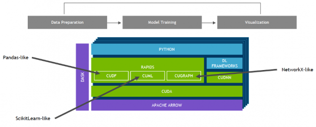
A general data science process and competition tip are to set up a fast experimentation pipeline on GPUs, where you train, improve the features and model, and then validate repeatedly. The NVIDIA team used a fast experimentation pipeline on GPUs consisting of preprocessing and feature engineering with RAPIDS cuDF, a library for GPU-accelerated dataframe transformations, combined with TensorFlow and PyTorch for deep learning. The RAPIDS suite of open-source software libraries, built on CUDA, gives you the ability to execute end-to-end data science and analytics pipelines entirely on GPUs, while still using familiar interfaces like Pandas and Scikit-Learn APIs.
Figure 4: End-to-End Data science pipeline with GPUs and RAPIDS.
Exploratory Data Analysis
Exploratory data analysis (EDA) is performed before, during, and after feature engineering to understand the dataset better. EDA uses data visualization, statistics, and queries to find important variables, interesting relations among the variables, anomalies, patterns, and insights.
The training dataset consists of a csv file with 1.5 million anonymized hotel reservations, based on real data, with the following features:
User_id – User ID
Check-in – Reservation check-in date
Checkout – Reservation check-out date
Affiliate_id – An anonymized ID of affiliate channels where the booker came from (e.g. direct, some third-party referrals, paid search engine, etc.)
Device_class – desktop/mobile
Booker_country – Country from which the reservation was made (anonymized)
Hotel_country – Country of the hotel (anonymized)
City_id – city_id of the hotel’s city (anonymized)
Utrip_id – Unique identification of user’s trip (a group of multi-destination bookings within the same trip)
Each reservation is a part of a customer’s trip (identified by utrip_id) which includes at least 4 consecutive reservations. The evaluation dataset is constructed similarly, however the city_id of the final reservation of each trip is concealed and requires a prediction.
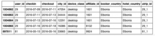
The sequence of user trip reservations can be obtained by sorting on the user_id and check-in date. Below, we read in the train and test data from the csv files using cuDF, sort on the userid, check-in date to obtain the sequence of trip reservations for a user. A count on the sorted dataset reveals 269k trips.
train = cudf.read_csv('../00_Data/booking_train_set.csv').sort_values(by=['user_id','checkin'])
test = cudf.read_csv('../00_Data/booking_test_set.csv').sort_values(by=['user_id','checkin'])


print(train.shape, test.shape)
train.head()
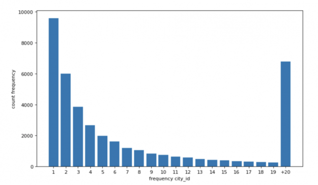
Visualizing the data can help with preprocessing and feature selection by revealing trends in the data. Histograms or bar charts help visualize the distribution of a feature. For example, the count vs. the city id frequency chart below shows that the distribution of the city reservation frequency was long-tailed as one would expect – some cities are much more popular for tourism and business than others. To help the models to focus less on very unpopular cities (city reservation frequency
Figure 5: Distribution of frequency of city_id in train and test dataset. Around 10,000 city ids appeared only once in the dataset.
Feature Pre-Processing, Selection, and Generation
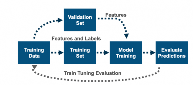
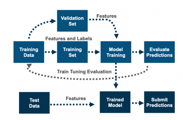
Feature engineering and feature selection is an iterative process that starts with engineering new features, then training a model, and then evaluating the model predictions against the target labels. The goal is to determine which features improve the model’s prediction accuracy. You repeat this process, along with hyperparameter tuning, until you are satisfied with the model’s accuracy.
Figure 6: Machine learning is an iterative process involving feature engineering, training, testing, and tuning.
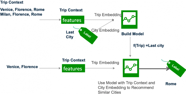
Framing this problem under the recommender systems taxonomy, the cities are the items we want to recommend for a trip. The trip is analogous to a session in the session-based recommendation task (see part 2 of this series), which is generally a sequence of user interactions – city hotel reservations in this case.
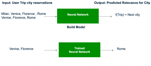
Figure 7: The recommender model learns the trip and city embeddings based on the trip features and last city (label) which are then used by the trained model to infer similar next cities.
Feature generation creates new features using knowledge about the problem and data. Feature columns can be combined, subtracted, counted, aggregated, and transformed to create new features to describe the user session (the Trip) and the cities. The NVIDIA team created the following additional features from the original 9:
Trip context date, time features: day-of-week, week-of-year, month, weekend, season, stay length (checkout – check-in), days since the last booking (check-in – previous checkout).
Trip context sequence features: the first city in the trip, lagged (previous 5) cities and countries from the trip.
Trip context statistics: trip length (number of reservations), trip duration (days), reservation order (in ascending and descending orders).
Past user trip statistics: number of user’s past reservations, number of user’s past trips, number of user’s past visited cities, number of user’s past visited countries.
Geographic seasonal city popularity: features based on the conditional probabilities of a city c from a country co, being visited at a month m or at a week-of-year w, as follows: P(c | m), P(c | m, co), P(c | w), P(c | w, co).
The dataset with 1.5M bookings is relatively small in comparison to other recommendation datasets. Techniques were explored to increase the training data by data augmentation and the team discovered that doubling the dataset with reversed trips improved the model’s accuracy. A trip is an ordered sequence of cities and although there are many permutations to visit a set of cities, there is a logical ordering implied by distances between cities and available transportation connections. These characteristics are commutative. For example, a trip of Boston->New York->Princeton->Philadelphia->Washington DC can be booked in reverse order, but not many people would book in a random order like Boston->Princeton->Washington DC->New York->Philadelphia.
Machine Learning Algorithms Used by the Winning Team
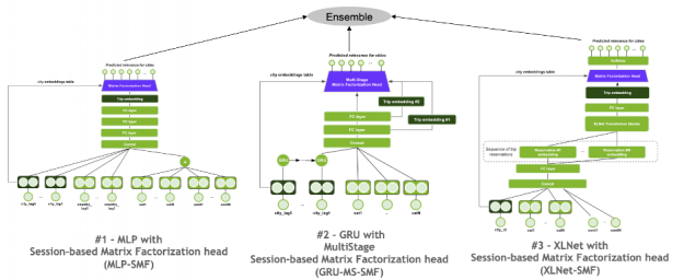
Ensemble methods combine multiple machine learning algorithms to obtain a better model. For the winning solution, the final submission was a simple ensemble (weighted average) of the predictions from models of three different neural architectures: Multilayer perceptron with Session-based Matrix Factorization net (MLP-SMF), Gated Recurrent Unit with MultiStage Session-based Matrix Factorization net (GRU-MS-SMF), and XLNet (Transformer) with Session-based Matrix Factorization net (XLNet-SMF). As the cardinality of the label (city) is not large, all models treated the recommendation as a multi-class classification problem, by using softmax cross-entropy loss function.
In deep learning, the last layer of a neural network used for classification can often be interpreted as a logistic regression. In this context, one can see a deep learning algorithm as multiple feature learning stages, which then pass their features into a logistic regression that classifies an input. The softmax function is a generalization of logistic regression often used to normalize the output of a neural network to a probability distribution over predicted output classes for multi-class classification.
Figure 8: The final submission was an ensemble of the predictions from models of three different neural architectures.
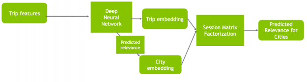
Session-based Matrix Factorization Layer
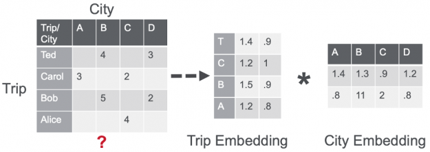
A shared component among the three different neural architectures was a Session-based Matrix Factorization (SMF) layer, which learns a linear mapping between the item (city) embeddings and the session (trip) embeddings to generate recommendations (the scores (logits) for cities) by a dot product operation.
Figure 9: A shared component among the three architectures was a Session-based Matrix Factorization layer.
This design was inspired by the MF-based Collaborative Filtering (see part 1), which learns latent factors for users and items by performing a dot product of their embeddings to predict the relevance of an item for a user.
Figure 10: Matrix factorization factors a sparse user item interaction matrix R (u-by-i) into a u-by-f matrix (U) and a f-by-i matrix (I). In this case the user is the trip session and the item is the city.
The large majority of users had only a single trip available in the dataset. So, instead of trying to model the user preference, the last layer of the network is used to represent the session (trip) embedding. Then, the dot product is computed between the session embedding s and all the set I of item embeddings i, where i is an element of I, to model items relevance probability distribution r of each item (city) being the next for that session (trip), such as r = softmax(s * I).
MLP with Session-based Matrix Factorization head (MLP-SMF)
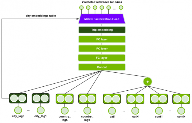
The MLP with Session-based Matrix Factorization head (MLP-SMF) uses feedforward and embedding layers, as seen in Figure 11.
Figure 11: MLP-SMF model architecture.
Categorical input features are fed through an embedding layer and continuous input features are individually projected via a linear layer to embeddings, followed by batch normalization and ReLU non-linear activation. All embedding dimensions are made equal. The embeddings of continuous input features and categorical input features, except the lag features, are combined via summation. The output is concatenated with the embeddings of the 5 last cities and countries (lag features).
The embedding tables for the city lags are shared, and similarly for hotel country lags. The lag embeddings are concatenated, but the model should still be able to learn the sequential patterns of cities by the order of lag features, i.e., city lag1’s embedding vector is always in the same position of the concatenated vector. The concatenated vector is fed through 3 feed-forward layers with batch normalization, PReLU activation function and dropout, to form the session (trip) embedding. It is used by the Session-based Matrix Factorization head to produce the scores for all cities.
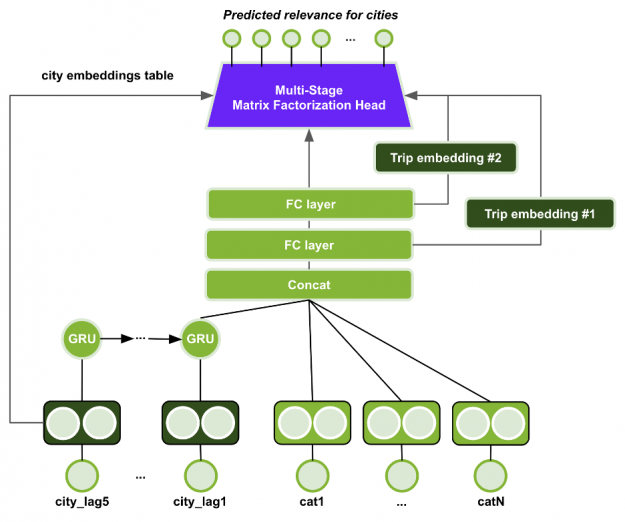
GRU with MultiStage Session-based Matrix Factorization head (GRU-MS-SMF)
The GRU with MultiStage Session-based Matrix Factorization head uses a GRU cell for embedding the historical user actions (previous 5 visited cities), similar to GRU4Rec. (see part 2 for more information on GRUs and session based recommenders). Missing values (sequences with less than 5 length) are padded with 0s. The last GRU hidden state is concatenated with the embeddings of the other categorical input features, as shown in Figure 12.
Figure 12: GRU-MS-SMF model architecture.
The embedding tables for the previous cities are shared. The model uses only categorical input features, including some numerical features modeled as embeddings such as trip length and reservation order. The concatenated embeddings are fed through a MultiStage Session-based Matrix Factorization head. The first stage in the MS-SMF is a softmax head over all items, which is used to select the top-50 cities for the next stage. In the second stage, the Session-based Matrix Factorization head is applied using only the top-50 cities of the first stage and two representations of the trip embeddings (the outputs of the last and second-to-last MLP layers, after the concatenation), resulting in two additional heads. The final output is a weighted sum of all three heads, with trainable weights. The multi-stage head works as a 2-stage ranking problem. The first head ranks all items and the other two heads can focus on the reranking of the top-50 items from the first stage. This approach can potentially scale to large item catalogs, i.e., in the order of millions. This dataset did not require such scalability, but this multi-stage design might be effective for deployment in production.
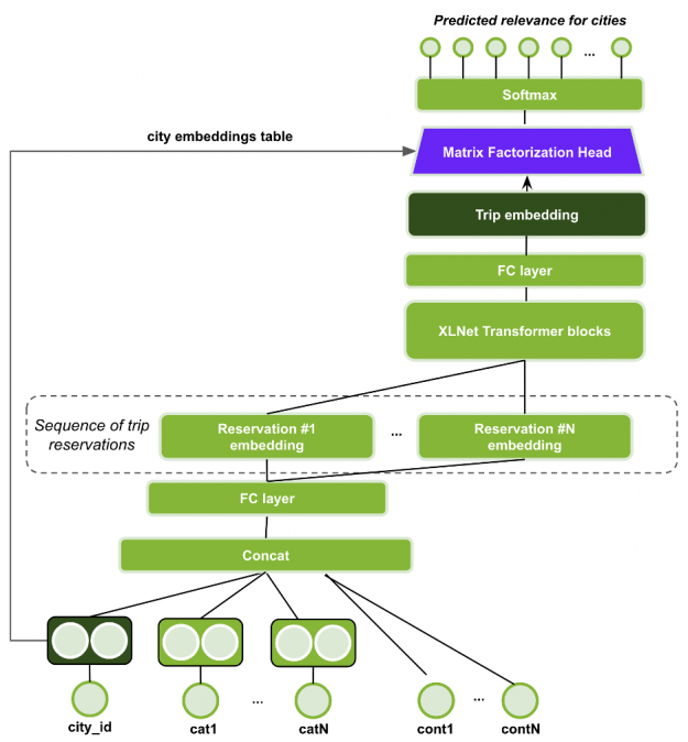
XLNet with Session-based Matrix Factorization head (XLNet-SMF)
The XLNet with Session-based Matrix Factorization head (XLNet-SMF) uses a Transformer architecture named XLNet, originally proposed for the permutation-based language modeling task in Natural Language Processing (NLP). In this case, the sequence of items in the session (trip) are modeled instead of the sequence of word tokens (see part 2 for more information on transformers and session based recommenders).
Figure 13: XLNet-SMF model architecture.
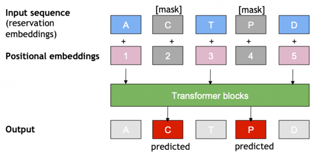
The XLNet training task was adapted for Masked Language Modeling (also known as Cloze task), like proposed by BERT4Rec for sequential recommendation. In that approach, for each training step, a proportion of all items are masked from the input sequence (i.e., replaced with a single trainable embedding), and then the original ids of the masked items are predicted using other items of the sequence, from both left and right sides. When a masked item is not the last one, this approach allows the usage of privileged information of the future reservations in the trip during training. Therefore, during inference, only the last item of the sequence is masked, to match the sequential recommendation task and to not leak future information of the trip.
Figure 14: During masked language sequence model training, the model is allowed to use items on the right (future information) for predictions. During evaluation, the last item of the sequence is masked to prevent future information leak.
For this network, each example is a trip, represented as a sequence of its reservations. The reservation embedding is generated by concatenating the features and projecting using MLP layers. The sequence of reservation embeddings is fed to the XLNet Transformer stacked blocks, in which the output of each block is the input of the next block. The final transformer block output generates the trip embedding.
Finally, the Matrix Factorization head (dot product between the trip embedding and city embeddings) is used to produce a probability distribution over the cities for the masked items in the sequence.
Evaluating the Model
To evaluate a model’s accuracy, you test the model’s predictions, in this case the final city (city_id) of each trip, against the labeled outcome. To do this, you split the training dataset, which has labeled data, train the model on part of the data, and evaluate the predictions with the rest. For this competition, the evaluation metric was Precision@4. Precision at 4 corresponds to the proportion of top-scoring results that are relevant, in this case scoring as correct if the top-4 recommendations include the last city.
Training and Hyperparameter Tuning
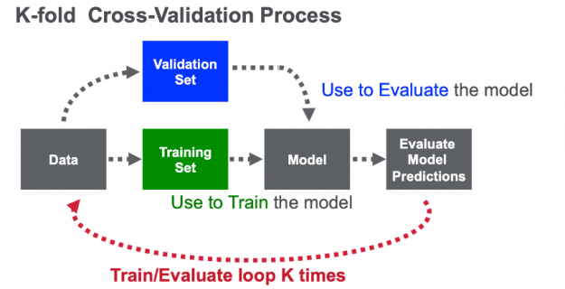
Unlike most competitions, this competition allowed only two submissions (predictions on the unlabeled test file). Because it was key to select the best features, hyperparameters and models for the final submission, it was crucial to design a good validation set. For this reason the team used k-fold cross validation, a method that maximizes the training dataset for training, tuning and evaluating a model. With cross-validation, the data is randomly split into k partitions (folds). Each fold is used one time as the validation dataset, while the rest (Out-Of-Fold – OOF) are used for training. Models are trained using the OOF training sets and evaluated with the validation sets, resulting in k model accuracy measurements.
Figure 15. With k-fold cross-validation, the data is split into k folds (partitions). Each fold is used one time as the validation dataset, while the rest (Out-Of-Fold – OOF) are used for training.
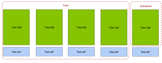
The NVIDIA team used 5-fold cross validation, using both the train data (from train.csv) and test data (test.csv), this is unusual since the test.csv data does not have the final city, but it does have a sequence of cities. For each fold, the fold train data was used for evaluation and data (both train and test) from the other folds (Out-Of-Fold – OOF) was used to train the model. The full OOF dataset was used, predicting the last city given previous ones. The Cross-Validation (CV) score was the average Precision@4 from each of the five folds.
Figure 16: For each fold, the train set fold was used for evaluation and both the train and test set Out-Of-Folds for training.
Hyperparameter optimization tunes the model’s properties that can be set for training to find the most accurate possible model; for example the learning rate, learning rate decay, or batch size. The choice of optimal hyperparameters is between underfitting and overfitting a model—where the model predictions match how the training data behaves and is also generalized enough to make accurate predictions on unseen data. When working with neural networks, the choice of hyperparameters can make the difference between poor and superior predictive performance. To find out more about how the NVIDIA team tuned the model hyperparameters see the appendix in this whitepaper: Using Deep Learning to Win the Booking.com WSDM WebTour21 Challenge on Sequential Recommendations.
Ensembling
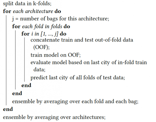
Ensembling is a proven approach to improve the accuracy of models, by combining their predictions and improving generalization. K-fold cross-validation and bagging techniques were used to ensemble models from the three architectures, as shown in Figure 17.
Figure 17: Ensemble Algorithm.
In general, the higher the diversity of the model’s predictions, the more the ensembling technique can potentially improve the final scores. In this case, the correlation of the predicted city scores between each two combinations of the three architectures was around 80%, which resulted in a representative improvement with ensembling in the final CV score.
Final Model Predictions Submission
The final step (which in this competition allowed only two submissions per team) was to submit the teams top four city predictions per each trip on the test set in a csv file named submission.csv with the following columns:
Figure 16. After feature engineering, training, and tuning, the final step is to submit predictions on the test data.
The NVIDIA team’s final leaderboard result was 0.5939 for precision@4 and scored 2.8% better than the second solution.
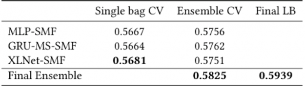
In order to clarify the contribution from each architecture and from the ensembling algorithm for the final result, the table below shows the cross-validation Precision@4 results by architecture, individual and after bagging ensembling, and the final ensemble from the three architectures combined. XLNet-SMF was the most accurate single model. The MLP-SMF architecture achieved a CV score comparable to the other two architectures that explicitly model the sequences using GRU and XLNet (Transformer). As the MLP-SMF model was lightweight, it was much faster to train than the other architectures, which sped up its experimentation cycle and improvements.
Figure 18. Final results by architecture and for the final ensemble – MLP-SMF uses 8 bags, GRU-MS-SMF uses 7 bags and XLNet-SMF uses 5 bags.
Summary
In this blog, we walked through the process of how NVIDIA’S team won the Booking.com WSDM WebTour 21 Challenge. We went over the domain problem, winning techniques in EDA, feature preprocessing, and generation, the DL models, and validation for improving predictions. The NVIDIA team designed three different deep learning architectures based on MLP, GRU, and Transformer neural building blocks. Some techniques resulted in improved performance for all models, like the Session-based Matrix Factorization head and the data augmentation with reversed trips. The diversity of the model architectures resulted in significant accuracy improvements by ensembling model predictions. We hope this post, the solution, and the links below, are useful to others interested in building recommendation systems.

 cuSOLVERMp provides a distributed-memory multi-node and multi-GPU solution for solving systems of linear equations at scale! In the future, it will also solve eigenvalue and singular value problems.


 Background Predictive maintenance is used for early fault detection, diagnosis, and prediction when maintenance is needed in various industries including oil and gas, manufacturing, and transportation. Equipment is continuously monitored to measure things like sound, vibration, and temperature to alert and report potential issues. To accomplish this in computers, the first step is to determine …
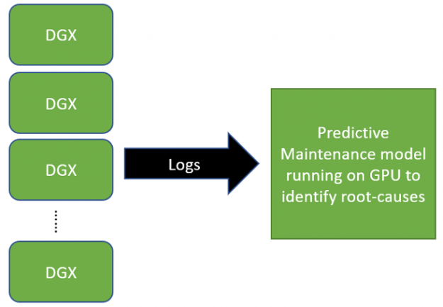
 Recently, at GTC21, the NVIDIA CloudXR team ran a Connect with Experts session about the CloudXR SDK. We shared how CloudXR can deliver limitless virtual and augmented reality over networks (including 5G) to low cost, low-powered headsets and devices, all while maintaining the high-quality experience traditionally reserved for high-end headsets that are plugged into high-performance …


 Recommender systems (RecSys) have become a key component in many online services, such as e-commerce, social media, news service, or online video streaming. However with the growth in importance, the growth in scale of industry datasets, and more sophisticated models, the bar has been raised for computational resources required for recommendation systems. To meet the …