Jaguar Land Rover and NVIDIA are redefining modern luxury, infusing intelligence into the customer experience. As part of its Reimagine strategy, Jaguar Land Rover announced today that it will develop its upcoming vehicles on the full-stack NVIDIA DRIVE Hyperion 8 platform, with DRIVE Orin delivering a wide spectrum of active safety, automated driving and parking Read article >
However, from what I can observe so far, the tensorboard graph does not really indicate user-understandable node names and cell names which makes it so difficult for tracking down the connections within the graph.
Stepping deeper into the era of exascale AI, Atos gave the first look at its next-generation high-performance computer. The BullSequana XH3000 combines Atos’ patented fourth-generation liquid-cooled HPC design with NVIDIA technologies to deliver both more performance and energy efficiency. Giving users a choice of Arm or x86 computing architectures, it will come in versions using Read article >
Hi, I’m trying to train a GAN on the mnist fashion dataset. But whenever I train the thing it keeps returning each epoch
W tensorflow/core/data/root_dataset.cc:163] Optimization loop failed: CANCELLED: Operation was cancelled W tensorflow/core/data/root_dataset.cc:163] Optimization loop failed: CANCELLED: Operation was cancelled W tensorflow/core/data/root_dataset.cc:163] Optimization loop failed: CANCELLED: Operation was cancelled W tensorflow/core/data/root_dataset.cc:163] Optimization loop failed: CANCELLED: Operation was cancelled W tensorflow/core/data/root_dataset.cc:163] Optimization loop failed: CANCELLED: Operation was cancelled W tensorflow/core/data/root_dataset.cc:163] Optimization loop failed: CANCELLED: Operation was cancelled
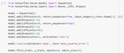
It doesn’t seem to actually train every time l look at the generated images. Here is the code:
Hey guys, i am struggling with the definition of the quantity of hidden layers of these RNN (see below). Contain this model three or two hidden LSTM-Layers? I’m not sure. Is the first LSTM-Layer simultan the Input-Layer or are there an additional Input Layer before the first LSTM-Layer?
HIII I HOPE SOMEONE CAN REALLY REALLY HELP ME WITH THIS:) Do I need to reduce dimension using LDA before passing it into my Tensorflow Training/testing model? I can’t really find any tensorflow lda function code online, I am currently using sk.learn’s LDA then pass the data into tensorflow. Is that ok? Or do I not even need to reduce dimensionality at all if I use tensorflow? 🙂 Thankssss
Posted by David Patterson, Distinguished Engineer, Google Research, Brain Team
Machine learning (ML) has become prominent in information technology, which has led some to raise concerns about the associated rise in the costs of computation, primarily the carbon footprint, i.e., total greenhouse gas emissions. While these assertions rightfully elevated the discussion around carbon emissions in ML, they also highlight the need for accurate data to assess true carbon footprint, which can help identify strategies to mitigate carbon emission in ML.
In “The Carbon Footprint of Machine Learning Training Will Plateau, Then Shrink”, accepted for publication in IEEE Computer, we focus on operational carbon emissions — i.e., the energy cost of operating ML hardware, including data center overheads — from training of natural language processing (NLP) models and investigate best practices that could reduce the carbon footprint. We demonstrate four key practices that reduce the carbon (and energy) footprint of ML workloads by large margins, which we have employed to help keep ML under 15% of Google’s total energy use.
The 4Ms: Best Practices to Reduce Energy and Carbon Footprints We identified four best practices that reduce energy and carbon emissions significantly — we call these the “4Ms” — all of which are being used at Google today and are available to anyone using Google Cloud services.
Model. Selecting efficient ML model architectures, such as sparse models, can advance ML quality while reducing computation by 3x–10x.
Machine. Using processors and systems optimized for ML training, versus general-purpose processors, can improve performance and energy efficiency by 2x–5x.
Mechanization. Computing in the Cloud rather than on premise reduces energy usage and therefore emissions by 1.4x–2x. Cloud-based data centers are new, custom-designed warehouses equipped for energy efficiency for 50,000 servers, resulting in very good power usage effectiveness (PUE). On-premise data centers are often older and smaller and thus cannot amortize the cost of new energy-efficient cooling and power distribution systems.
Map Optimization. Moreover, the cloud lets customers pick the location with the cleanest energy, further reducing the gross carbon footprint by 5x–10x. While one might worry that map optimization could lead to the greenest locations quickly reaching maximum capacity, user demand for efficient data centers will result in continued advancement in green data center design and deployment.
These four practices together can reduce energy by 100x and emissions by 1000x.
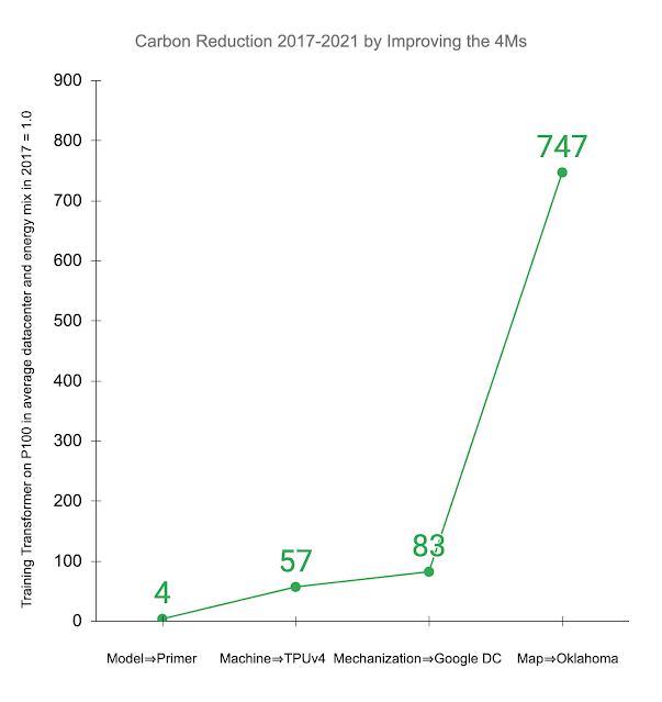
Below, we illustrate the impact of improving the 4Ms in practice. Other studies examined training the Transformer model on an Nvidia P100 GPU in an average data center and energy mix consistent with the worldwide average. The recently introduced Primer model reduces the computation needed to achieve the same accuracy by 4x. Using newer-generation ML hardware, like TPUv4, provides an additional 14x improvement over the P100, or 57x overall. Efficient cloud data centers gain 1.4x over the average data center, resulting in a total energy reduction of 83x. In addition, using a data center with a low-carbon energy source can reduce the carbon footprint another 9x, resulting in a 747x total reduction in carbon footprint over four years.
Reduction in gross carbon dioxide equivalent emissions (CO2e) from applying the 4M best practices to the Transformer model trained on P100 GPUs in an average data center in 2017, as done in other studies. Displayed values are the cumulative improvement successively addressing each of the 4Ms: updating the model to Primer; upgrading the ML accelerator to TPUv4; using a Google data center with better PUE than average; and training in a Google Oklahoma data center that uses very clean energy.
Overall Energy Consumption for ML Google’s total energy usage increases annually, which is not surprising considering increased use of its services. ML workloads have grown rapidly, as has the computation per training run, but paying attention to the 4Ms — optimized models, ML-specific hardware, efficient data centers — has largely compensated for this increased load. Our data shows that ML training and inference are only 10%–15% of Google’s total energy use for each of the last three years, each year split ⅗ for inference and ⅖ for training.
Prior Emission Estimates Google uses neural architecture search (NAS) to find better ML models. NAS is typically performed once per problem domain/search space combination, and the resulting model can then be reused for thousands of applications — e.g., the Evolved Transformer model found by NAS is open sourced for all to use. As the optimized model found by NAS is often more efficient, the one time cost of NAS is typically more than offset by emission reductions from subsequent use.
Without ready access to Google hardware or data centers, the study extrapolated from the available P100 GPUs instead of TPUv2s, and assumed US average data center efficiency instead of highly efficient hyperscale data centers. These assumptions increased the estimate by 5x over the energy used by the actual NAS computation that was performed in Google’s data center.
In order to accurately estimate the emissions for NAS, it’s important to understand the subtleties of how they work. NAS systems use a much smaller proxy task to search for the most efficient models to save time, and then scale up the found models to full size. The UMass study assumed that the search repeated full size model training thousands of times, resulting in emission estimates that are another 18.7x too high.
The overshoot for the NAS was 88x: 5x for energy-efficient hardware in Google data centers and 18.7x for computation using proxies. The actual CO2e for the one-time search were 3,223 kg versus 284,019 kg, 88x less than the published estimate.
Unfortunately, some subsequent papers misinterpreted the NAS estimate as the training cost for the model it discovered, yet emissions for this particular NAS are ~1300x larger than for training the model. These papers estimated that training the Evolved Transformer model takes two million GPU hours, costs millions of dollars, and that its carbon emissions are equivalent to five times the lifetime emissions of a car. In reality, training the Evolved Transformer model on the task examined by the UMass researchers and following the 4M best practices takes 120 TPUv2 hours, costs $40, and emits only 2.4 kg (0.00004 car lifetimes), 120,000x less. This gap is nearly as large as if one overestimated the CO2e to manufacture a car by 100x and then used that number as the CO2e for driving a car.
Outlook Climate change is important, so we must get the numbers right to ensure that we focus on solving the biggest challenges. Within information technology, we believe these are much more likely the lifecycle costs — i.e., emission estimates that include the embedded carbon emitted from manufacturing all components involved, from chips to data center buildings — of manufacturing computing equipment of all types and sizes1 rather than the operational cost of ML training.
Expect more good news if everyone improves the 4Ms. While these numbers may currently vary across companies, these simple measures can be followed across the industry:
If the 4Ms become widely recognized, we predict a virtuous circle that will bend the curve so that the global carbon footprint of ML training is actually shrinking, not increasing.
Acknowledgements Let me thank my co-authors who stayed with this long and winding investigation into a topic that was new to most of us: Jeff Dean, Joseph Gonzalez, Urs Hölzle, Quoc Le, Chen Liang, Lluis-Miquel Munguia, Daniel Rothchild, David So, and Maud Texier. We also had a great deal of help from others along the way for an earlier study that eventually led to this version of the paper. Emma Strubell made several suggestions for the prior paper, including the recommendation to examine the recent giant NLP models. Christopher Berner, Ilya Sutskever, OpenAI, and Microsoft shared information about GPT-3. Dmitry Lepikhin and Zongwei Zhou did a great deal of work to measure the performance and power of GPUs and TPUs in Google data centers. Hallie Cramer, Anna Escuer, Elke Michlmayr, Kelli Wright, and Nick Zakrasek helped with the data and policies for energy and CO2e emissions at Google.
1Worldwide IT manufacturing for 2021 included 1700M cell phones, 340M PCs, and 12M data center servers. ↩
At the latest UEFA Champions League Finals, one of the world’s most anticipated annual soccer events, pop stars Marshmello, Khalid and Selena Gomez shared the stage for a dazzling opening ceremony at Portugal’s third-largest football stadium — without ever stepping foot in it. The stunning video performance took place in a digital twin of the Read article >
Learn how the Time Series Prediction Platform provides an end-to-end framework that enables users to train, tune, and deploy time series models.
In this post, we detail the recently released NVIDIA Time Series Prediction Platform (TSPP), a tool designed to compare easily and experiment with arbitrary combinations of forecasting models, time-series datasets, and other configurations. The TSPP also provides functionality to explore the hyperparameter search space, run accelerated model training using distributed training and Automatic Mixed Precision (AMP), and deploy and run inference on accelerated model formats on the NVIDIA Triton Inference Server.
Accurately forecasting future time series values using previous values has proven pivotal in understanding and managing complex systems, including but not limited to power grids, supply chains, and financial markets. In these forecasting applications, single-digit percentage improvements in predictive accuracy can have vast financial, ecological, and social impacts. In addition to needing to be accurate, forecasting models also must be able to function on real-time timescale.
Figure 1: A depiction of the typical sliding-window time series forecasting problem. Each sliding window consists of time-sequential data that is split into two parts, the past, and the future.
The sliding window forecasting problem, shown preceding in Figure 1, involves using prior data and knowledge of future values to predict future target values. Traditional statistical methods, such as ARIMA and its variants, or Holt-Winters Regression have long been used to perform regression for these tasks. However, as data volume has increased and the problems to solve with regression have become increasingly complex, deep learning approaches have proven their ability to represent effectively and understand these problems.
Despite the advent of deep learning forecasting models, there historically has not been a way to effectively experiment with and compare the performance and accuracy of time series models across an arbitrary set of datasets. To this end, we’re delighted to publicly open-source the NVIDIA Time Series Prediction Platform.
What is the TSPP?
The Time Series Prediction Platform is an end-to-end framework that enables users to train, tune, and deploy time series models. Its hierarchical configuration system and rich feature specification API allow for new models, datasets, optimizers, and metrics to be easily integrated and experimented with. The TSPP is designed for use with vanilla PyTorch models and is agnostic to the cloud or local platforms.
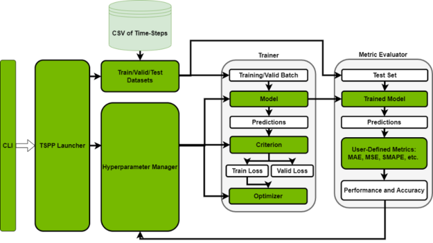
Figure 2: The basic architecture of the NVIDIA Time Series Prediction Platform. The CLI feeds the input to the TSPP launcher, which instantiates the objects required for training (model, dataset, etc.) and runs the specified experiment to generate performance and accuracy results.
The TSPP, pictured in Figure 2, is centered around a command line-controlled launcher. Based on user input to the CLI, the launcher either instantiates a hyperparameter manager, which can run a set of training experiments in parallel or will run a single experiment by creating the described components, such as model, dataset, metric, etc.
Models supported
The TSPP supports the NVIDIA Optimized Temporal Fusion Transformer (TFT) by default. Within the TSPP, TFT training can be accelerated using multi-GPU training, automatic mixed precision, and exponential moving weight averaging. The model can be deployed using the aforementioned inference and deployment pipeline.
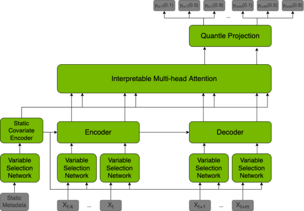
The TFT model is a hybrid architecture joining LSTM encoding and interpretable transformer attention layers. Prediction is based on three types of variables: static (constant for a given time series), known (known in advance for whole history and future), observed (known only for historical data). All of these variables come in two flavors: categorical, and continuous. In addition to historical data, we feed the model with historical values of the time series itself.
All variables are embedded in high-dimensional space by learning an embedding vector. Categorical variables embeddings are learned in the classical sense of embedding discrete values. The model learns a single vector for each continuous variable, which is then scaled by this variable’s value for further processing. The next step is to filter variables through the Variable Selection Network (VSN), which assigns weights to the inputs in accordance with their relevance to the prediction. Static variables are used as a context for variable selection of other variables and as an initial state of LSTM encoders.
After encoding, variables are passed to multi-head attention layers (decoder), which produce the final prediction. The whole architecture is interwoven with residual connections with gating mechanisms that allow the architecture to adapt to various problems.
Figure 3: Diagram of the TFT architecture: Bryan Lim, Sercan O. Arik, Nicolas Loeff, Tomas Pfister from Temporal Fusion Transformers for Interpretable Multi-horizon Time Series Forecasting, 2019.
Accelerated training
When experimenting with deep learning models, training acceleration can greatly increase the number of experimental iterations you can make in a given time. The Time Series Prediction Platform provides the ability to accelerate training with any combination of Automatic Mixed Precision, Multi-GPU Training, and Exponential Moving Weight Averaging.
Training quick start
Once one is inside the TSPP container, running the TSPP is as simple as calling the launcher with the combination of a dataset, model, and other components that you want to use. For example, to train TFT with the Electricity dataset, we simply call:
The resulting logs, checkpoints, and initial config will be saved to outputs. For examples that include more complex workflows, please reference the repository documentation.
Automatic mixed precision
Automatic Mixed Precision (AMP) is a mode of execution for deep learning training, where applicable calculations are computed in 16-bit precision instead of 32-bit precision. AMP execution can greatly accelerate deep learning training without loss of accuracy. AMP is included in the TSPP and can be enabled by simply adding a flag to the launch call.
Multi-GPU training
Multi-GPU data parallel training provides acceleration for model training by increasing the global batch size by running model computations in parallel on all available GPUs. This approach can greatly improve model training time without loss of model accuracy, especially when many GPUs are used. It is included in the TSPP through PyTorch DistributedDataParallel and can be enabled by simply adding an element to the launch call.
Exponential moving weight averaging
Exponential Moving Weight Averaging is a technique that maintains two copies of a model, one that is being trained through backpropagation, and a second model that is the weighted average of the weights of the first model. At test and inference time, the averaged weights are used to compute outputs. This approach has proven to decrease time to convergence and increase convergence accuracy in practice, at the cost of doubling model GPU memory requirements. EMWA is included in the TSPP and can be enabled by simply adding a flag to the launch call.
Hyperparameter tuning
Model hyperparameter tuning is an essential part of the model development and experimentation process for deep learning models. For this purpose, the TSPP includes a rich integration with the Optuna hyperparameter search library. Users can run extensive hyperparameter searches by specifying hyperparameter names and distributions to search on. Once this is done, the TSPP can run multi-GPU or single-GPU trials in parallel until the desired number of hyperparameter options have been explored.
At search completion, the TSPP will return the hyperparameters of the best single run, as well as the log files of all runs. For ease of comparison, the log files are generated with the NVIDIA DLLogger and are easily searchable and compatible with Tensorboard plotting.
Configurability
Configurability in the TSPP is driven by Hydra, an open-source library provided by Facebook. Hydra allows users to define a hierarchical configuration system using YAML files that are combined at runtime, making launching runs as simple as stating ‘I want to try this model with this dataset’.
Feature specification
The feature specification, which is included in the dataset portion of configuration, is a standard description language for time-series datasets. It encodes the attributes of each tabular feature with information about whether it is known, observed, or static in the future, whether or not the feature is categorical or continuous, and many more optional attributes. This description language provides a framework for models to automatically configure themselves based on arbitrary described input.
Component integration
Adding a new dataset to the TSPP is as simple as creating a feature specification for it and describing the dataset itself. Once the feature specification and a few other key values have been defined, models integrated with the TSPP will be able to configure themselves to the new dataset.
Adding a new model to the TSPP simply requires that the model expects the data presented by the feature specification to be in the correct channel. If the model correctly interprets the feature spec, the model should work with all datasets integrated into the TSPP, past, and future.
In addition to models and datasets, the TSPP also supports the integration of arbitrary components, such as criterion, optimizers, and goal metrics. Through the use of Hydra’s direct instantiation of objects using config, users can integrate their own custom components and use them simply using the specification in a launch of the TSPP.
Inference and deployment
Inference is a key component of any Machine Learning pipeline. To this end, the TSPP has built-in support for inference that integrates seamlessly with the platform. In addition to supporting native inference, the TSPP also supports single-step deployment of converted models to NVIDIA Triton Inference Servers.
NVIDIA Triton model navigator
The TSPP provides full support for the NVIDIA Triton Model Navigator. Compatible models can be easily converted to optimized formats including TorchScript, ONNX, and NVIDIA TensorRT. In the same step, these converted models will be deployed to an NVIDIA Triton Inference Server. There is even an option to profile, analyze, and generate helm charts for a given model as part of a single step. For example, given a TFT output folder, we can convert and deploy a model to NVIDIA TensorRT format in fp16 by exporting to ONNX with the following command:
We benchmarked TFT within the TSPP on two datasets: the Electrical Load (Electricity) dataset from the UCI dataset repository, and the PEMs Traffic dataset (Traffic). TFT achieves strong results on both datasets, achieving the lowest seen error on both datasets and confirming the assessment of the authors of the TFT paper.
Dataset
Mean Absolute Error
Root Mean Squared Error
Electricity
43.807
142307.152
Traffic
0.005081
0.018
Table 1:
Training Performance
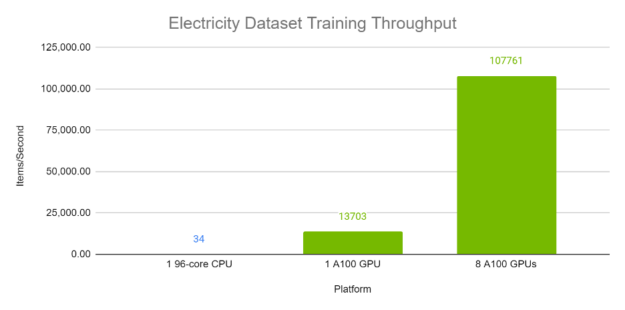
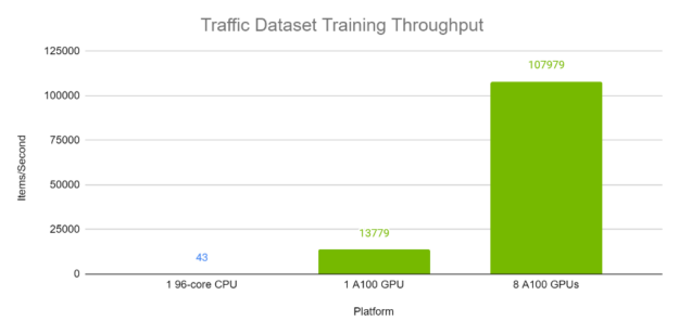
Figures 4 and 5 demonstrate the per-second throughput of TFT on the Electricity and Traffic datasets respectively. Each batch, with batch size 1024, contains a variety of time windows from different time series within the same dataset. The A100 runs were computed using Automatic Mixed Precision. As is evident, TFT has excellent performance and scaling on A100 GPUs, especially when compared with execution on a 96-core CPU.
Figure 4: TFT training throughput on Electricity dataset on GPU versus CPU. GPUs: 8x Tesla A100 80 GB. CPU: Intel(R) Xeon(R) Platinum 8168 CPU @ 2.70GHz (96 threads).
Figure 5. TFT training throughput on Traffic dataset on GPU versus CPU. GPUs: 8x Tesla A100 80 GB. CPU: Intel(R) Xeon(R) Platinum 8168 CPU @ 2.70GHz (96 threads).
Training time
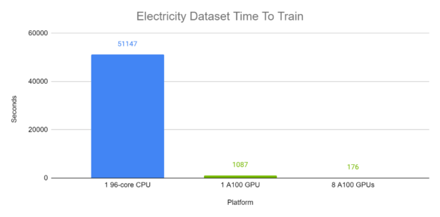
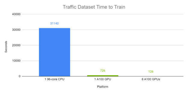
Figures 6 and 7 demonstrate the end-to-end training time of TFT on the Electricity and Traffic datasets respectively. Each batch, with batch size 1024, contains a variety of time windows from different time series within the same dataset. The A100 completed runs were computed using Automatic Mixed Precision. In these experiments, on GPU, TFT is trained in minutes, while the CPU runs trained in approximately half a day.
Figure 6: TFT end-to-end training time on Electricity dataset on GPU compared to CPU. GPUs: 8x Tesla A100 80 GB. CPU: Intel(R) Xeon(R) Platinum 8168 CPU @ 2.70GHz (96 threads).
Figure 7: TFT end-to-end training time on Traffic dataset on GPU compared to CPU. GPUs: 8x Tesla A100 80 GB. CPU: Intel(R) Xeon(R) Platinum 8168 CPU @ 2.70GHz (96 threads).
Inference Performance
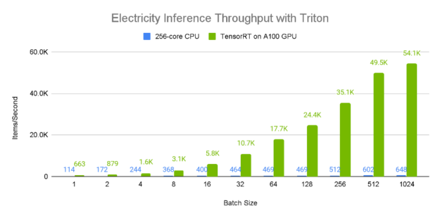
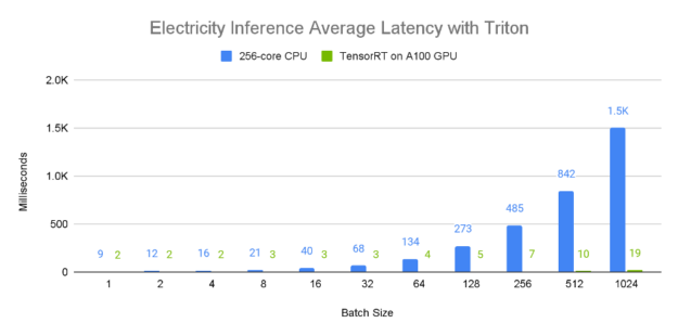
Figures 8 and 9 demonstrate the relative single-device inference throughput and average latency of an A100 80GB GPU vs a 96-core CPU across a variety of batch sizes on the electricity dataset. Since larger batch sizes generally generate greater inference throughput, we consider the 1024 element batch results, where it is apparent that the A100 GPU has incredible performance, processing approximately 50,000 samples a second. Furthermore, larger batch sizes tend to lead to higher latency as is evident from the CPU values, which seem to scale proportionally with the batch size. In contrast, the A100 GPU has a near constant average latency when compared to the CPU.
Figure 8: TFT throughput on Electricity dataset when deployed to NVIDIA Triton Inference Server Container 21.12 on GPU vs CPU. GPUs: 1x Tesla A100 80 GB deployed using TensorRT 8.2. CPU: Dual AMD Rome 7742, 128 cores total @ 2.25 GHz (base), 3.4 GHz (max boost) (256 threads) deployed using ONNX.
Figure 9: TFT average latency on Electricity dataset when deployed to NVIDIA Triton Inference Server Container 21.12 on GPU vs CPU. GPUs: 1x Tesla A100 80 GB deployed using TensorRT 8.2. CPU: Dual AMD Rome 7742, 128 cores total @ 2.25 GHz (base), 3.4 GHz (max boost)(256 threads) deployed using ONNX.
End-to-end example
Tying together the preceding examples, we demonstrate a simple training and deployment of the TFT model on the Electricity dataset. We begin by building and launching the TSPP container from the source:
cd DeeplearningExamples/Tools/PyTorch/TimeSeriesPredictionPlatform
source scripts/setup.sh
docker build -t tspp .
docker run -it --gpus all --ipc=host --network=host -v /your/datasets/:/workspace/datasets/ tspp bash
Next, we launch the TSPP with the electricity dataset, TFT, and a quantile loss. We also overload the number of epochs to train for 10. Once the model has been trained, logs, config files, and a trained checkpoint will be created in outputs/{date}/{time}, in this case, outputs/01-02-2022/:
The NVIDIA Time Series Prediction Platform provides end-to-end GPU acceleration from training to inference for time series models. The reference example included in the platform is optimized and certified to run on NVIDIA DGX A100 and NVIDIA-Certified Systems. For a deeper dive into the performance achieved see our Temporal Fusion Transformer benchmarks.
Organizations can start training, comparing model architectures with their own datasets, and deploying the models in production today.
Secure, robust, tinyML based delivery of agricultural products to its valid consumers is the most important step for our AREC.
Secure, robust delivery of agricultural products to its valid consumers is the most important step for our AREC-Agricultural Records on Electronic Contracts solution. Not only it should be streamed toward getting accurate regional data analytics but should also make it nearly impossible to counterfeit goods, I took up this challenge because I am very aware of the situation in India, for example: during Covid-19 fake pesticides made up almost a quarter of the market exposing Himachal Pradesh farmers, their apple crops and the environment to many harmful side effects.
One of the biggest reasons behind the growth of fake products in the agrochemical industry is the lack of knowledge about genuine products among consumers. Illiterate farmers usually do not check the product authentication features and just go for the cheap price.
Rare adoption of anti-counterfeiting solutions by companies: Many agrochemical manufacturers do not implement anti-counterfeiting solutions in their products. This makes their products highly susceptible to duplication, tampering and even diversion.
Lack of stringent regulatory measures: Lack of strict regulatory measures against counterfeit products and poor laws against counterfeiters has led to the rapid rise of counterfeit agro-chemical products. Challenge: Develop an easily accessible solution for farmers that can provide detailed product-specific information, their usage, and the delivery details, and help them increase productivity and profitability.
Our idea is to bring a secure de-centralized, tamperproof unified blockchain ledger with a secure authentication device protocol to streamline all manufacturers and logistics data. The device sends and updates the following data to the ledger:
location
temp&humidity
seal/packet opened or not
tinyML based condition status (For instance, if there is a sudden change in temperature that would damage the goods – abnormal environmental conditions during transit of agrochemicals like pesticides can result in separation of active ingredients, a notification is sent that triggers an action to resolve the situation.)
Using the device ID barcode, the farmer can scan and get to know all details, in fact, it would be one time process to onboard the farmer to the Blockchain ledger, the product ID barcode would serve as farmer login and it would allow him to trace and lodge complain in case of any unsatisfactory results.
Used on a variety of зкщвгсеы – Information will be presented on the packaging. (Taking into account a variety of products (crop protection and seeds) and packaging (eg bags, 250ml, 20L, etc).
Customers can scan/read and interact with the Digital Label
Provides simple and actionable information about seeds, traits, and crop protection products
Uses scannable resources like QR codes to provide information about the product (nutrients and pesticides) like geography, dosage, applicability, authenticity, usage, and disposal guidelines
Supports customer feedback, and complaints – Customers can communicate with the company regarding a specific product
Can create a dynamic label that can be adjusted to cover important legal requirements like safety statements and product’s identification information
Product traceability (localization and expected delivery date- information flow from farmer to customers)
Provides product security, or anti-counterfeiting – Making sure that the product is not forged/Copied and is an original company product.
Has flexible Data Model to support the different data inputs and maintenance, since we need to keep legal requirements data, label artwork models, product usage data, product data, security data, delivery data, etc.
To build flexible and extensible data/information models that can handle vast and diverse information related to individual products.
Technology Overview:
MCU choice: Our application requires robust performance over a long time more than 6 months with minimum power consumption (here, focused on driving down cost, power consumption and size so 8bit MCU would be a great option too).
tinyML framework choice: Recently, explored the Neuton ai platform and was blown away by the flexibility it provides for embedding huge ML models with lower memory footprints even on an 8bit MCU. The training is easy with greatly optimized C codes for MCUs. It offers various model explainability tools that allow users to evaluate the trained model quality and understand the cause of prediction for the inference data.
Blockchain frameworkchoice:Daml idea is to abstract the key concepts of blockchains that allow them to provide consistency guarantees on distributed systems of record. Daml, a virtual shared ledger, governed by smart contracts, takes the place of a concrete blockchain. Adding this layer of abstraction allows Daml to realize a whole range of capabilities and advantages that are sorely lacking in individual blockchain and distributed ledger technologies.
Fleet Monitoring: There are several reasons to consider this to allow better regulation of tracking devices. I have tried Golioth and Toit and both seem to be fantastic in terms of security and visibility but I will lean more towards C/C++ support. (I will work on this in future)
Below is what our label would look like and the essential data printed on it. It would only contain a battery, microprocessor, SIM, modem and antenna under its unassuming surface.
Testing DAML blockchain with our product (I used toit to test a use case for fleet monitoring and remote logging), check the below images for understanding our Blockchain ledger pipeline. With blockchain, we have selected visibility of immutable data which can be accessed under specific roles by scanning a QR code on the label.
Than I build the model using Neuton Platfrom
Building TinyML model for our smart labels in 3 steps:
Step 1: Creating Solution and Adding Dataset
Step 2: TinyML model setting and Training
Our model has Coefficients: 120 Model Size Kb: 0.46 File Size for Embedding Kb: 0.553, pretty tiny and smart 🙂
Step 3: Make Predictions on MCUs


 Learn how the Time Series Prediction Platform provides an end-to-end framework that enables users to train, tune, and deploy time series models.
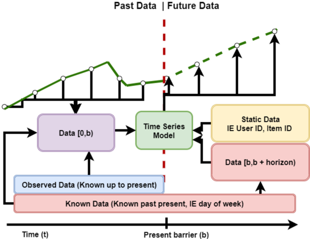

