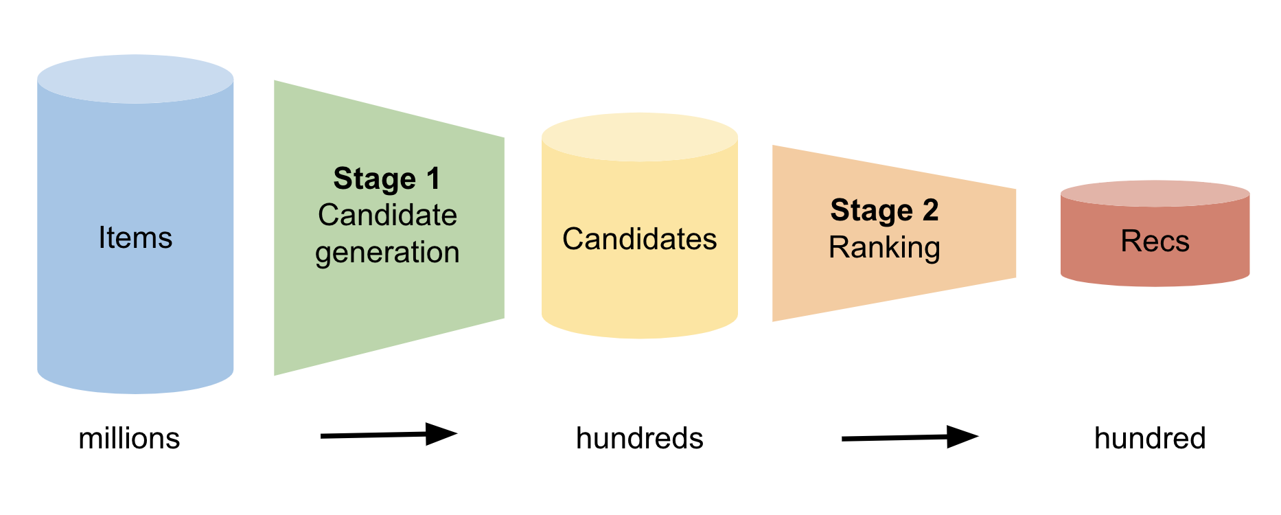
Reading has many benefits for young students, such as better linguistic and life skills, and reading for pleasure has been shown to correlate with academic success. Furthermore students have reported improved emotional wellbeing from reading, as well as better general knowledge and better understanding of other cultures. With the vast amount of reading material both online and off, finding age-appropriate, relevant and engaging content can be a challenging task, but helping students do so is a necessary step to engage them in reading. Effective recommendations that present students with relevant reading material helps keep students reading, and this is where machine learning (ML) can help.
ML has been widely used in building recommender systems for various types of digital content, ranging from videos to books to e-commerce items. Recommender systems are used across a range of digital platforms to help surface relevant and engaging content to users. In these systems, ML models are trained to suggest items to each user individually based on user preferences, user engagement, and the items under recommendation. These data provide a strong learning signal for models to be able to recommend items that are likely to be of interest, thereby improving user experience.
In “STUDY: Socially Aware Temporally Causal Decoder Recommender Systems”, we present a content recommender system for audiobooks in an educational setting taking into account the social nature of reading. We developed the STUDY algorithm in partnership with Learning Ally, an educational nonprofit, aimed at promoting reading in dyslexic students, that provides audiobooks to students through a school-wide subscription program. Leveraging the wide range of audiobooks in the Learning Ally library, our goal is to help students find the right content to help boost their reading experience and engagement. Motivated by the fact that what a person’s peers are currently reading has significant effects on what they would find interesting to read, we jointly process the reading engagement history of students who are in the same classroom. This allows our model to benefit from live information about what is currently trending within the student’s localized social group, in this case, their classroom.
Data
Learning Ally has a large digital library of curated audiobooks targeted at students, making it well-suited for building a social recommendation model to help improve student learning outcomes. We received two years of anonymized audiobook consumption data. All students, schools and groupings in the data were anonymized, only identified by a randomly generated ID not traceable back to real entities by Google. Furthermore all potentially identifiable metadata was only shared in an aggregated form, to protect students and institutions from being re-identified. The data consisted of time-stamped records of student’s interactions with audiobooks. For each interaction we have an anonymized student ID (which includes the student’s grade level and anonymized school ID), an audiobook identifier and a date. While many schools distribute students in a single grade across several classrooms, we leverage this metadata to make the simplifying assumption that all students in the same school and in the same grade level are in the same classroom. While this provides the foundation needed to build a better social recommender model, it’s important to note that this does not enable us to re-identify individuals, class groups or schools.
The STUDY algorithm
We framed the recommendation problem as a click-through rate prediction problem, where we model the conditional probability of a user interacting with each specific item conditioned on both 1) user and item characteristics and 2) the item interaction history sequence for the user at hand. Previous work suggests Transformer-based models, a widely used model class developed by Google Research, are well suited for modeling this problem. When each user is processed individually this becomes an autoregressive sequence modeling problem. We use this conceptual framework to model our data and then extend this framework to create the STUDY approach.
While this approach for click-through rate prediction can model dependencies between past and future item preferences for an individual user and can learn patterns of similarity across users at train time, it cannot model dependencies across different users at inference time. To recognise the social nature of reading and remediate this shortcoming we developed the STUDY model, which concatenates multiple sequences of books read by each student into a single sequence that collects data from multiple students in a single classroom.
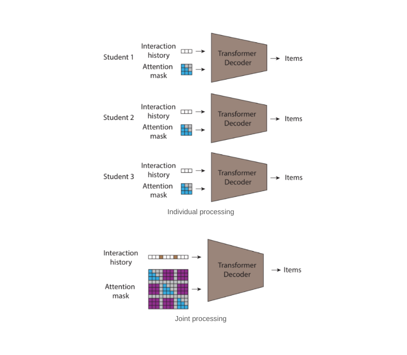
However, this data representation requires careful diligence if it is to be modeled by transformers. In transformers, the attention mask is the matrix that controls which inputs can be used to inform the predictions of which outputs. The pattern of using all prior tokens in a sequence to inform the prediction of an output leads to the upper triangular attention matrix traditionally found in causal decoders. However, since the sequence fed into the STUDY model is not temporally ordered, even though each of its constituent subsequences is, a standard causal decoder is no longer a good fit for this sequence. When trying to predict each token, the model is not allowed to attend to every token that precedes it in the sequence; some of these tokens might have timestamps that are later and contain information that would not be available at deployment time.
 |
| In this figure we show the attention mask typically used in causal decoders. Each column represents an output and each column represents an output. A value of 1 (shown as blue) for a matrix entry at a particular position denotes that the model can observe the input of that row when predicting the output of the corresponding column, whereas a value of 0 (shown as white) denotes the opposite. |
The STUDY model builds on causal transformers by replacing the triangular matrix attention mask with a flexible attention mask with values based on timestamps to allow attention across different subsequences. Compared to a regular transformer, which would not allow attention across different subsequences and would have a triangular matrix mask within sequence, STUDY maintains a causal triangular attention matrix within a sequence and has flexible values across sequences with values that depend on timestamps. Hence, predictions at any output point in the sequence are informed by all input points that occurred in the past relative to the current time point, regardless of whether they appear before or after the current input in the sequence. This causal constraint is important because if it is not enforced at train time, the model could potentially learn to make predictions using information from the future, which would not be available for a real world deployment.
 |
| In (a) we show a sequential autoregressive transformer with causal attention that processes each user individually; in (b) we show an equivalent joint forward pass that results in the same computation as (a); and finally, in (c) we show that by introducing new nonzero values (shown in purple) to the attention mask we allow information to flow across users. We do this by allowing a prediction to condition on all interactions with an earlier timestamp, irrespective of whether the interaction came from the same user or not. |
<!–
 |
| In (a) we show a sequential autoregressive transformer with causal attention that processes each user individually; in (b) we show an equivalent joint forward pass that results in the same computation as (a); and finally, in (c) we show that by introducing new nonzero values (shown in purple) to the attention mask we allow information to flow across users. We do this by allowing a prediction to condition on all interactions with an earlier timestamp, irrespective of whether the interaction came from the same user or not. |
–><!–
 |
| In (a) we show a sequential autoregressive transformer with causal attention that processes each user individually; in (b) we show an equivalent joint forward pass that results in the same computation as (a); and finally, in (c) we show that by introducing new nonzero values (shown in purple) to the attention mask we allow information to flow across users. We do this by allowing a prediction to condition on all interactions with an earlier timestamp, irrespective of whether the interaction came from the same user or not. |
–>
Experiments
We used the Learning Ally dataset to train the STUDY model along with multiple baselines for comparison. We implemented an autoregressive click-through rate transformer decoder, which we refer to as “Individual”, a k-nearest neighbor baseline (KNN), and a comparable social baseline, social attention memory network (SAMN). We used the data from the first school year for training and we used the data from the second school year for validation and testing.
We evaluated these models by measuring the percentage of the time the next item the user actually interacted with was in the model’s top n recommendations, i.e., hits@n, for different values of n. In addition to evaluating the models on the entire test set we also report the models’ scores on two subsets of the test set that are more challenging than the whole data set. We observed that students will typically interact with an audiobook over multiple sessions, so simply recommending the last book read by the user would be a strong trivial recommendation. Hence, the first test subset, which we refer to as “non-continuation”, is where we only look at each model’s performance on recommendations when the students interact with books that are different from the previous interaction. We also observe that students revisit books they have read in the past, so strong performance on the test set can be achieved by restricting the recommendations made for each student to only the books they have read in the past. Although there might be value in recommending old favorites to students, much value from recommender systems comes from surfacing content that is new and unknown to the user. To measure this we evaluate the models on the subset of the test set where the students interact with a title for the first time. We name this evaluation subset “novel”.
We find that STUDY outperforms all other tested models across almost every single slice we evaluated against.
 |
| In this figure we compare the performance of four models, Study, Individual, KNN and SAMN. We measure the performance with hits@5, i.e., how likely the model is to suggest the next title the user read within the model’s top 5 recommendations. We evaluate the model on the entire test set (all) as well as the novel and non-continuation splits. We see STUDY consistently outperforms the other three models presented across all splits. |
Importance of appropriate grouping
At the heart of the STUDY algorithm is organizing users into groups and doing joint inference over multiple users who are in the same group in a single forward pass of the model. We conducted an ablation study where we looked at the importance of the actual groupings used on the performance of the model. In our presented model we group together all students who are in the same grade level and school. We then experiment with groups defined by all students in the same grade level and district and also place all students in a single group with a random subset used for each forward pass. We also compare these models against the Individual model for reference.
We found that using groups that were more localized was more effective, with the school and grade level grouping outperforming the district and grade level grouping. This supports the hypothesis that the STUDY model is successful because of the social nature of activities such as reading — people’s reading choices are likely to correlate with the reading choices of those around them. Both of these models outperformed the other two models (single group and Individual) where grade level is not used to group students. This suggests that data from users with similar reading levels and interests is beneficial for performance.
Future work
This work is limited to modeling recommendations for user populations where the social connections are assumed to be homogenous. In the future it would be beneficial to model a user population where relationships are not homogeneous, i.e., where categorically different types of relationships exist or where the relative strength or influence of different relationships is known.
Acknowledgements
This work involved collaborative efforts from a multidisciplinary team of researchers, software engineers and educational subject matter experts. We thank our co-authors: Diana Mincu, Lauren Harrell, and Katherine Heller from Google. We also thank our colleagues at Learning Ally, Jeff Ho, Akshat Shah, Erin Walker, and Tyler Bastian, and our collaborators at Google, Marc Repnyek, Aki Estrella, Fernando Diaz, Scott Sanner, Emily Salkey and Lev Proleev.
 Optical Character Detection (OCD) and Optical Character Recognition (OCR) are computer vision techniques used to extract text from images. Use cases vary across…
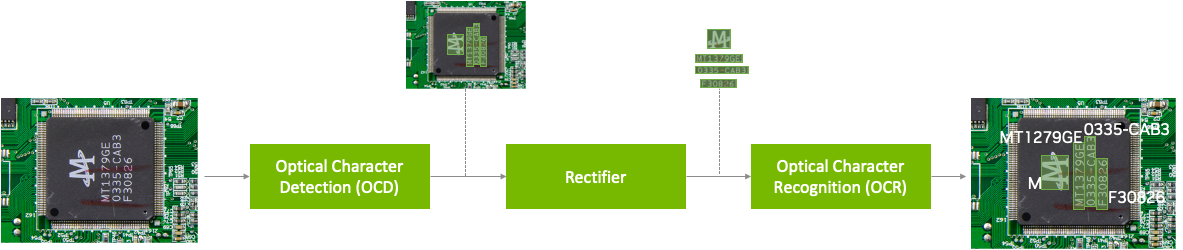

 NVIDIA Triton Inference Server streamlines and standardizes AI inference by enabling teams to deploy, run, and scale trained ML or DL models from any framework…
 Explore the latest streaming analytics features and advancements with this new release.
 Next-generation AI pipelines have shown incredible success in generating high-fidelity 3D models, ranging from reconstructions that produce a scene matching…

 Soccer is considered one of the most popular sports around the world. And with good reason: the action is often intense, and the game combines both physicality…
 Picture this: You’re browsing through an online store, looking for the perfect pair of running shoes. But with thousands of options available, where do you even…