NVIDIA will be presenting a new paper introducing a new method for generating level-of-detail of complex models, taking both geometry and surface appearance into account.
NVIDIA will be presenting a new paper titled “Appearance-Driven Automatic 3D Model Simplification” at Eurographics Symposium on Rendering 2021 (EGSR), June 29-July 2, introducing a new method for generating level-of-detail of complex models, taking both geometry and surface appearance into account.
Level-of-detail for aggregate geometry, where we represent each leaf as a semi-transparent textured quad. The geometrical complexity is greatly reduced, to just 0.4% of the original triangle count, with little visual impact.
Level-of-detail has long been used in computer games as a means of improving performance and reducing aliasing artifacts that may occur due to shading detail or small geometric features. Traditional approaches to level of detail include mesh simplification, normal map baking, and shading/BSDF prefiltering. Each problem is typically tackled in isolation.
We approach level-of-detail entirely in image space, with our optimization objective being “does a simplified model look like the reference when rendered from a certain distance?” (i.e., we use a standard image loss). This perspective is not entirely new, but recent advances in differentiable rendering have transformed it from a theoretical exercise to something highly practical, with excellent performance. We propose an efficient inverse rendering method and system that can be used to simultaneously optimize shape and materials to generate level-of-detail models, or clean up the result of automatic simplification tools.
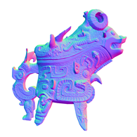
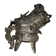
Approaching model simplification through inverse rendering lets us unify previous methods into a single system, optimizing for a single loss. This is important, because the system can negotiate which rendering term is best suited to represent a detail. An example is shown in the image below, where we create a simplified version of the Ewer statue. By using normal mapping in the inverse rendering setup, the system automatically determines which features are best represented by geometry, and which can be represented by the normal map.
Normal Map
Our (7k tris)
Reference (300k tris)
We show that our method is applicable to a wide range of applications including level-of-detail, normal and displacement map baking, shape and appearance prefiltering and simplification of aggregate geometry, all while supporting animated geometry. We can additionally convert between surface representations, e.g. convert an implicit surface to a mesh, different material representations and different renderers.
Refer to the paper and supplemental material for full results. Our source code is publicly available at GitHub.
Today, NVIDIA is releasing a SIGGRAPH 2021 technical paper, “Real-time Neural Radiance Caching for Path Tracing” that introduces another leap forward in real-time global illumination: Neural Radiance Caching. Global illumination, that is, illumination due to light bouncing around in a scene, is essential for rich, realistic visuals. This is a challenging task, even in cinematic … Continued
Today, NVIDIA is releasing a SIGGRAPH 2021 technical paper, “Real-time Neural Radiance Caching for Path Tracing” that introduces another leap forward in real-time global illumination: Neural Radiance Caching.
Global illumination, that is, illumination due to light bouncing around in a scene, is essential for rich, realistic visuals. This is a challenging task, even in cinematic rendering, because it is difficult to find all the paths of light that contribute meaningfully to an image. Solving this problem through brute force requires hundreds, sometimes thousands of paths per pixel, but this is far too expensive for real-time rendering.
Direct illumination alone (left) lacks indirect reflections. Global illumination (right) adds indirect reflections, resulting in refined image detail and realism. The images were rendered offline.
Before NVIDIA RTX introduced real-time ray tracing to games, global illumination in games was largely static. Since then, technologies such as RTXGI bring dynamic global illumination to life. They overcome the limited realism of pre-computing “baked” lighting in dynamic worlds and simplify an otherwise tedious lighting design process.
Neural Radiance Caching combines RTX’s neural network acceleration hardware (NVIDIA TensorCores) and ray tracing hardware (NVIDIA RTCores) to create a system capable of fully-dynamic global illumination that works with all kinds of materials, be they diffuse, glossy, or volumetric. It handles fine-scale textures such as albedo, roughness, or bump maps, and scales to large, outdoor environments neither requiring auxiliary data structures nor scene parameterizations.
Combined with NVIDIA’s state-of-the-art direct lighting algorithm, ReSTIR, Neural Radiance Caching can improve rendering efficiency of global illumination by up to a factor of 100—two orders of magnitude.
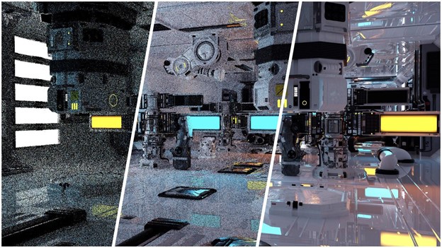
NVIDIA’s combination of ReSTIR and Neural Radiance Caching (middle) exhibits less noise than path tracing (left). The right image shows an offline rendered ground truth.
NVIDIA’s combination of ReSTIR and Neural Radiance Caching (middle) exhibits less noise than path tracing (left). The right image shows an offline rendered ground truth.
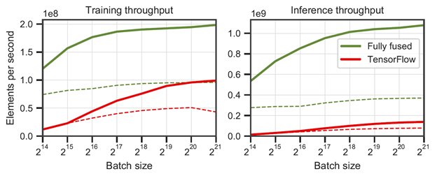
At the heart of the technology is a single tiny neural network that runs up to 9x faster than TensorFlow v2.5.0. Its speed makes it possible to train the network live during gameplay in order to keep up with arbitrary dynamic content. On an NVIDIA RTX 3090 graphics card, Neural Radiance Caching can provide over 1 billion global illumination queries per second.
NVIDIA’s fully fused neural networks outperforming TensorFlow v2.5.0 for a 64 neuron wide (solid line) and 128 neuron wide (dashed line) multi-layer perceptrons on an NVIDIA RTX 3090.
NVIDIA’s fully fused neural networks outperforming TensorFlow v2.5.0 for a 64 neuron wide (solid line) and 128 neuron wide (dashed line) multi-layer perceptrons on an NVIDIA RTX 3090.
Training is often considered an offline process with only inference occurring at runtime. In contrast, Neural Radiance Caching performs both training and inference at runtime, showing that real-time training of neural networks is practical.
This paper paves the way for using dynamic neural networks in various other areas of computer graphics and possibly other real-time fields, such as wireless communication and reinforcement learning.
“Our work represents a paradigm shift from complex, memory-intensive auxiliary data structures to generic, compute-intensive neural representations” says Thomas Müller, one of the paper’s authors. “Computation is significantly cheaper than memory transfers, which is why real-time trained neural networks make sense despite their massive number of operations.”
We are excited about future applications enabled by tiny real-time-trained neural networks and look forward to further research of real-time machine learning in computer graphics and beyond. To help researchers and developers adopt the technology, NVIDIA releases the CUDA source code of their tiny neural networks.
Researchers at NVIDIA presented a new paper “An Analytic BRDF for Materials with Spherical Lambertian Scatterers” at Eurographics Symposium on Rendering 2021 (EGSR), June 29-July 2, introducing a new BRDF for dusty/diffuse surfaces. Most rough diffuse BRDFs such as Oren-Nayar are based on a random height-field microsurface, which limits the range of roughnesses that are … Continued
Our new Lambert-sphere BRDF (right) accurately and efficiently models the reflectance of a porous microstructure consisting of Lambertian spherical particles.
Most rough diffuse BRDFs such as Oren-Nayar are based on a random height-field microsurface, which limits the range of roughnesses that are physically plausible (a height field can only get so spiky before it becomes implausible). To avoid this limitation and extend the usable range of rough diffuse BDRFs, we take a volumetric approach to surface microstructure to derive BRDF for very rough diffuse materials. It is simple and intuitive to control with a single diffuse color parameter and it produces more saturated colors and backscattering than other models.
The intersection of volume and surface representations in computer graphics is seeing a rapid growth with new techniques such as NeRF. Our ability to seamlessly interchange between surface and volume descriptions of the same scene with no noticeable appearance change is an important tool for efficiently authoring and rendering complex scenes. A BRDF is one such form of representation interchange. In this case, we derive the BRDF that simulates a porous volumetric microstructure consisting of Lambertian spherical particles (pictured above). In some sense this results in an infinitely rough version of the Oren-Nayar BRDF. The resulting BRDF can be used to render diffuse porous materials such as foam up to 100 times more efficiently than using stochastic random walk methods.
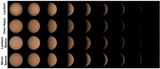
Our new Lambert-sphere BRDF produces brighter backscattering and more saturated rim lighting than other diffuse BRDFs.
We call our BRDF the Lambert-sphere (LS) BRDF. We present a highly accurate version that is only 30% slower to evaluate than Oren-Nayar, and a faster approximate version for real-time applications. We also include importance sampling for the Lambertian-sphere phase function for use rendering large diffusive smoke and debris particles. Below we compare our BRDF to Lambertian, Oren-Nayar and Chandrasekhar’s BRDF that consists of a thick volumetric layer of mirror spheres in an absorbing matrix.
NVIDIA researchers will present their paper “An Unbiased Ray-Marching Transmittance Estimator” at SIGGRAPH 2021, August 9-13, showing a new way to compute visibility in scenes with complex volumetric effects.
NVIDIA researchers will present their paper “An Unbiased Ray-Marching Transmittance Estimator” at SIGGRAPH 2021, August 9-13, showing a new way to compute visibility in scenes with complex volumetric effects.
We present new methods for reducing a common source of noise in scenes with volumetric effects.
When Monte Carlo sampling is used to compute lighting effects such as soft shadows and global illumination, shadow rays are used to query the visibility between lights and surfaces. In many scenes, visibility is a simple binary answer that is efficiently queried using the RTX RT Cores. However, for volumetric effects such as clouds, smoke and explosions, visibility is a fractional quantity ranging from 0.0 to 1.0, and computing this quantity efficiently and accurately between any two points in a scene is an essential part of photorealistic real-time rendering. Visibility that accounts for volumetric effects is also called transmittance.
We present a new algorithm, which we call unbiased ray marching, for evaluating this transmittance in general scenes. Our key result is a new statistically-unbiased Monte Carlo method that randomly queries the volume densities along a ray and computes a visibility estimate from these values. For high-performance rendering, the goal is to compute an accurate low-noise estimate while minimizing the number of times the volume data needs to be accessed.
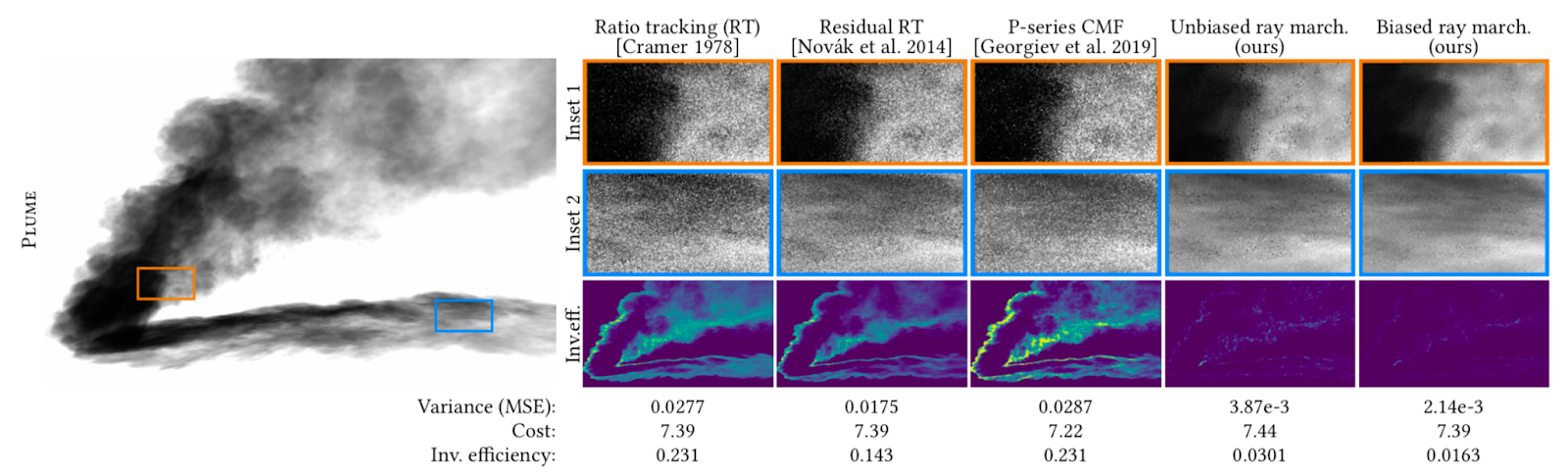
The research paper provides a new efficiency analysis of the transmittance estimation problem. This yields a number of key insights about when and how various transmittance estimators achieve the optimal balance of low noise and low cost. Building on these insights, and leveraging previous work from graphics, physics and statistics, we derive a new transmittance estimator that is universally optimal relative to 50 years of prior art, and often ten times more efficient than earlier methods. Technically, the end result is based on a power-series expansion of the exponential function that appears in the transmittance equation, and 90% of the time our new estimator simply evaluates the first term in this expansion. This first term corresponds to the traditional biased ray-marching algorithm. The subsequent terms of the expansion, which our estimator evaluates 10% of the time, correct for the bias. This key insight allows us to benefit from the efficiency of ray marching without being plagued by its bias – occasional light-leaking artifacts seen as, for example, overly bright clouds.
The new method helps to reduce the noise of shadows, such as the one cast on the floor by the smoke plume in the above figure where we see a dramatic reduction in noise at the same render time.
Putting a new twist on an old method, unbiased ray marching virtually eliminates a common source of noise in path-traced renderings of scenes with rich volumetric effects.
In this month’s technical digest we’re highlighting this powerful capability and offer a collection of resources to help ROS users familiarize with the power of Jetson, ISAAC SDK, ISAAC Sim and a success story from NVIDIA Inception Member, Aerobotics.
While you are likely already familiar with Jetson as the NVIDIA AI platform for edge AI, you might be surprised to learn that the power of Jetson isn’t limited to solutions built entirely on Jetson platforms. Jetpack on Jetson and Isaac SDK, our robotics platform, adds AI capabilities to existing autonomous machines and bridges dependencies for diverse hardware and software solutions.
In this month’s technical digest, we’re highlighting this powerful capability and offering a collection of resources to help Robotic Operating System (ROS) users get familiar with the power of Jetson, Isaac SDK, Isaac Sim, and a success story on a startup in the NVIDIA Inception program.
Jetson and ROS tutorials
Accelerating AI Modules for ROS and ROS 2 on NVIDIA Jetson Platform A showcase of support for ROS and ROS 2 on NVIDIA Jetson developer kits. Read now >
Building Robotics Applications Using ROS and NVIDIA Isaac SDK Learn how to use a ROS application stack with NVIDIA Isaac and ISAAC Sim. Read now >
Implementing Robotics Applications with ROS 2 and AI on the NVIDIA Jetson Platform Learn how to perform classification, object detection and pose estimation with ROS 2 on Jetson. Read now >
Top 5 Jetson resources
Meet Jetson, the platform for AI at the edge NVIDIA Jetson is used by professional developers to create breakthrough AI products across all industries, and by students and enthusiasts for hands-on AI learning and making amazing projects. Meet Jetson >
Getting started with Jetson Developer Kits Jetson developer kits are used by professionals to develop and test software for products based on Jetson modules, and by students and enthusiasts for projects and learning. Each developer kit includes a non-production specification Jetson module attached to a reference carrier board with standard hardware interfaces for flexible development and rapid prototyping. Learn more >
Free 8-hour class on getting started with AI on Jetson Nano In this course, you’ll use Jupyter iPython notebooks on your own Jetson Nano to build a deep learning classification project with computer vision models. Upon completion, you receive a certificate. Start learning hands-on today >
Jetson and Embedded Systems developer forums The Jetson and Embedded Systems community is active, vibrant, and continually monitored by the Jetson Product and Engineering teams. Meet the community >
Jetson community projects Explore and learn from Jetson projects created by us and our community. Explore community projects >
Recommended hardware
Jetson Nano 2GB Most affordable At 457 GFLOPs for $59, this developer kit is the ultimate starter AI computer. Learn more >
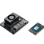
Jetson Xavier NX Great for multiple use cases Run modern neural networks and advanced AI applications within the footprint of a credit card. Learn more >
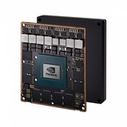
Partner solutions Production-ready now Our ecosystem partners can support subsystem designs all the way up to fully realized autonomous machines with their associated requirements. Learn more >
Inception spotlight
Bilberry: Using Jetson for Computer Vision for Crop Surveying In 2016, the former dormmates at École Nationale Supérieure d’Arts et Métiers in Paris, founded Bilberry. The startup developed a solution to recognize weeds powered by the NVIDIA Jetson edge AI platform for precision application of herbicides at corn and wheat farms, offering as much as a 92% reduction in herbicide usage. Learn more >
Do you have a startup? Join NVIDIA Inception’s global network of over 7,500 AI and data science startups.
Built with Enterprise IT Partners and Deployed First at Equinix, NVIDIA AI LaunchPad Includes End-to-End NVIDIA Hardware and Software Stack to Accelerate AI from Hybrid Cloud to EdgeSANTA …
SaaS Platform Helps Leading Device Makers, Factories, Warehouses and Retailers Deploy AI Products and ServicesSANTA CLARA, Calif., June 22, 2021 (GLOBE NEWSWIRE) — NVIDIA today announced …
Tackling one of the largest computing challenges of this lifetime requires larger than life computing. At CVPR this week, Andrej Karpathy, senior director of AI at Tesla, unveiled the in-house supercomputer the automaker is using to train deep neural networks for Autopilot and self-driving capabilities. The cluster uses 720 nodes of 8x NVIDIA A100 Tensor Read article >
File “c:UsersLandenOneDriveDesktopSign Language DetectorRealTimeObjectDetectionTensorflowscriptsgenerate_tfrecord.py”, line 62, in <module> label_map_dict = label_map_util.get_label_map_dict(label_map) File
“C:UsersLandenAppDataLocalProgramsPythonPython39libsite-packagesobject_detectionutilslabel_map_util.py”, line 164, in get_label_map_dict label_map = load_labelmap(label_map_path) File
“C:UsersLandenAppDataLocalProgramsPythonPython39libsite-packagesobject_detectionutilslabel_map_util.py”, line 133, in load_labelmap label_map_string = fid.read() File “C:UsersLandenAppDataLocalProgramsPythonPython39libsite-packagestensorflowpythonlibiofile_io.py”, line 117, in read self._preread_check() File
“C:UsersLandenAppDataLocalProgramsPythonPython39libsite-packagestensorflowpythonlibiofile_io.py”, line 79, in _preread_check self._read_buf = _pywrap_file_io.BufferedInputStream( TypeError: __init__(): incompatible constructor arguments.
In NVIDIA Clara Train 4.0, we added homomorphic encryption (HE) tools for federated learning (FL). HE enables you to compute data while the data is still encrypted. In Clara Train 3.1, all clients used certified SSL channels to communicate their local model updates with the server. The SSL certificates are needed to establish trusted communication … Continued
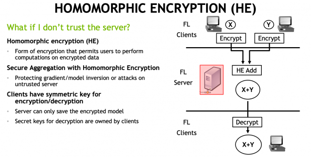
In NVIDIA Clara Train 4.0, we added homomorphic encryption (HE) tools for federated learning (FL). HE enables you to compute data while the data is still encrypted.
In Clara Train 3.1, all clients used certified SSL channels to communicate their local model updates with the server. The SSL certificates are needed to establish trusted communication channels and are provided through a third party that runs the provisioning tool and securely distributes them to the hospitals. This secures the communication to the server, but the server can still see the raw model (unencrypted) updates to do aggregation.
With Clara Train 4.0, the communication channels are still established using SSL certificates and the provisioning tool. However, each client optionally also receives additional keys to homomorphically encrypt their model updates before sending them to the server. The server doesn’t own a key and only sees the encrypted model updates.
With HE, the server can aggregate these encrypted weights and then send the updated model back to the client. The clients can decrypt the model weights because they have the keys and can then continue with the next round of training (Figure 1).
Figure 1. Why homomorphic encryption?
HE ensures that each client’s changes to the global model stays hidden by preventing the server from reverse-engineering the submitted weights and discovering any training data. This added security comes at a computational cost on the server. However, it can play an important role in healthcare in making sure that patient data stays secure at each hospital while still benefiting from using federated learning with other institutions.
These settings are recommended and should work for most tasks but could be further optimized depending on your specific model architecture and machine learning problem. For more information about different settings, see this tutorial on the CKKS scheme and benchmarking.
HE benchmarking in FL
To compare the impact of HE to the overall training time and performance, we ran the following experiments. We chose SegResNet (a U-Net like architecture used to win the BraTS 2018 challenge) trained on the CT spleen segmentation task from the Medical Segmentation Decathlon.
Each federated learning run was trained for 100 rounds with each client training for 10 local epochs on their local data on an NVIDIA V100 (server and clients are running on localhost). In each run, half of the clients each used half of the training data (16/16) and half of the validation data (5/4), respectively. We recorded the total training time and best average validation dice score of the global model. We show the relative increase added by HE in Table 1.
There is a moderate increase in total training time of about 20% when encrypting the full model. This increase in training time is due to the added encryption and decryption steps and aggregation in homomorphically encrypted space. Our implementation enables you to reduce that extra time by only encrypting a subset of the model parameters, for example, all convolutional layers (“conv”). You could also encrypt just three of the key layers, such as the input, middle, and output layers.
The added training time is also due to increased message sizes needed to send the encrypted model gradient updates, requiring longer upload times. For SegResNet, we observe an increase from 19 MB to 283 MB using the HE setting mentioned earlier (~15x increase).
Setting
Message size (MB)
Nr. clients
Training time
Best global Dice
Best epoch
Re. Increase in training time
Raw
19
2
4:57:26
0.951
931
–
Raw
19
4
5:11:20
0.956
931
–
Raw
19
8
5:18:00
0.943
901
–
HE full
283
2
5:57:05
0.949
931
20.1%
HE full
283
4
6:00:05
0.946
811
15.7%
HE full
283
8
6:21:56
0.963
971
20.1%
HE conv layers
272
2
5:54:39
0.952
891
19.2%
HE conv layers
272
4
6:06:13
0.954
951
17.6%
HE conv layers
272
8
6:28:16
0.948
891
22.1%
HE three layers
43
2
5:12:10
0.957
811
5.0%
HE three layers
43
4
5:15:01
0.939
841
1.2%
HE three layers
43
8
5:19:02
0.949
971
0.3%
Table 1. Relative increase in training time by running FL with secure aggregation using HE.
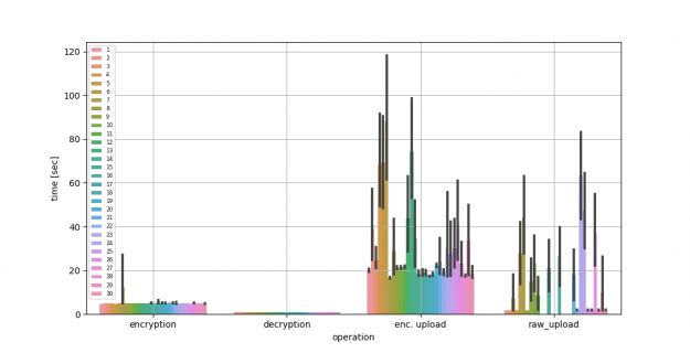
Next, we compare the performance of FL using up to 30 clients with the server running on AWS. For reference, we used an m5a.2xlarge with eight vCPUs, 32-GB memory, and up to 2,880 Gbps network bandwidth. We show the average encryption, decryption, and upload time, comparing raw compared to encrypted model gradients being uploaded in Figure 2 and Table 2. You can see the longer upload times due to the larger message sizes needed by HE.
Figure 2. Running federated learning with 30 clients and the server on AWS
Time in seconds
Mean
Std. Dev.
Encryption time
5.01
1.18
Decryption time
0.95
0.04
Enc. upload time
38
71.170
Raw upload time
21.57
74.23
Table 2. Federated learning using homomorphic encrypted compared to raw model updates.
Try it out
If you’re interested in learning more about how to set up FL with homomorphic encryption using Clara Train, we have a great Jupyter notebook on GitHub that walks you through the setup.
HE can reduce model inversion or data leakage risks if there is a malicious or compromised server. However, your final models might still contain or memorize privacy-relevant information. That’s where differential privacy methods can be a useful addition to HE. Clara Train SDK implements the sparse vector technique (SVT) and partial model sharing that can help preserve privacy. For more information, see Privacy-preserving Federated Brain Tumour Segmentation. Keep in mind that there is a tradeoff between model performance and privacy protection.

 NVIDIA will be presenting a new paper introducing a new method for generating level-of-detail of complex models, taking both geometry and surface appearance into account.
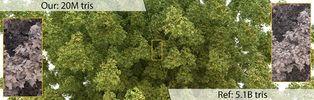

 Today, NVIDIA is releasing a SIGGRAPH 2021 technical paper, “Real-time Neural Radiance Caching for Path Tracing” that introduces another leap forward in real-time global illumination: Neural Radiance Caching. Global illumination, that is, illumination due to light bouncing around in a scene, is essential for rich, realistic visuals. This is a challenging task, even in cinematic …
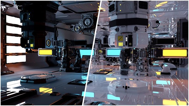
 Researchers at NVIDIA presented a new paper “An Analytic BRDF for Materials with Spherical Lambertian Scatterers” at Eurographics Symposium on Rendering 2021 (EGSR), June 29-July 2, introducing a new BRDF for dusty/diffuse surfaces. Most rough diffuse BRDFs such as Oren-Nayar are based on a random height-field microsurface, which limits the range of roughnesses that are …
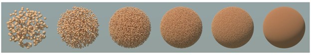
 NVIDIA researchers will present their paper “An Unbiased Ray-Marching Transmittance Estimator” at SIGGRAPH 2021, August 9-13, showing a new way to compute visibility in scenes with complex volumetric effects.
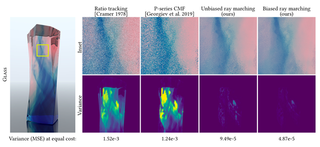
 In this month’s technical digest we’re highlighting this powerful capability and offer a collection of resources to help ROS users familiarize with the power of Jetson, ISAAC SDK, ISAAC Sim and a success story from NVIDIA Inception Member, Aerobotics.
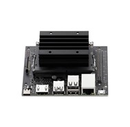
 In NVIDIA Clara Train 4.0, we added homomorphic encryption (HE) tools for federated learning (FL). HE enables you to compute data while the data is still encrypted. In Clara Train 3.1, all clients used certified SSL channels to communicate their local model updates with the server. The SSL certificates are needed to establish trusted communication …