
Organizations across industries are using extended reality (XR) to redesign workflows and boost productivity, whether for immersive training or collaborative design reviews. With the growing use of all-in-one (AIO) headsets, more teams have adopted and integrated XR. While easing XR use, AIO headsets have modest compute and rendering power that can limit the graphics quality Read article >
Machine learning helped Waseem Alshikh plow through textbooks in college. Now he’s putting generative AI to work, creating content for hundreds of companies. Born and raised in Syria, Alshikh spoke no English, but he was fluent in software, a talent that served him well when he arrived at college in Lebanon. “The first day they Read article >
Categories
NVIDIA CEO Brings Generative AI to SIGGRAPH
As generative AI continues to sweep an increasingly digital, hyperconnected world, NVIDIA founder and CEO Jensen Huang made a thunderous return to SIGGRAPH, the world’s premier computer graphics conference. “The generative AI era is upon us, the iPhone moment if you will,” Huang told an audience of thousands Tuesday during an in-person special address in Read article >
NVIDIA today announced the next-generation NVIDIA GH200 Grace Hopper™ platform — based on a new Grace Hopper Superchip with the world’s first HBM3e processor — built for the era of accelerated computing and generative AI.
NVIDIA and Hugging Face today announced a partnership that will put generative AI supercomputing at the fingertips of millions of developers building large language models (LLMs) and other advanced AI applications.
New Developer Toolkit Introduces Simplified Model Tuning and Deployment on NVIDIA AI Platforms — From PCs and Workstations to Enterprise Data Centers, Public Clouds and NVIDIA DGX CloudLOS …
NVIDIA and global manufacturers today announced powerful new NVIDIA RTX™ workstations designed for development and content creation in the age of generative AI and digitalization.
OVX Servers Feature New NVIDIA GPUs to Accelerate Training and Inference, Graphics-Intensive Workloads; Coming Soon From Dell Technologies, Hewlett Packard Enterprise, Lenovo, Supermicro and …
New Platform Updates, Connections to Adobe Firefly, OpenUSD to RealityKit, Ada-Generation Systems Accelerate Interoperable 3D Workflows and Industrial DigitalizationLOS ANGELES, Aug. 08, 2023 …
 Generative AI has introduced a new era in computing, one promising to revolutionize human-computer interaction. At the forefront of this technological marvel…
Generative AI has introduced a new era in computing, one promising to revolutionize human-computer interaction. At the forefront of this technological marvel are large language models (LLMs), empowering enterprises to recognize, summarize, translate, predict, and generate content using large datasets. However, the potential of generative AI for enterprises comes with its fair share of challenges.
Cloud services powered by general-purpose LLMs provide a quick way to get started with generative AI technology. However, these services are often focused on a broad set of tasks and are not trained on domain-specific data, limiting their value for certain enterprise applications. This leads many organizations to build their own solutions—a difficult task—as they must piece together various open-source tools, ensure compatibility, and provide their own support.
NVIDIA NeMo provides an end-to-end platform designed to streamline LLM development and deployment for enterprises, ushering in a transformative age of AI capabilities. NeMo equips you with the essential tools to create enterprise-grade, production-ready custom LLMs. The suite of NeMo tools simplifies the process of data curation, training, and deployment, facilitating the swift development of customized AI applications tailored to each organization’s specific requirements.
For enterprises banking on AI for their business operations, NVIDIA AI Enterprise presents a secure, end-to-end software platform. Combining NeMo with generative AI reference applications and enterprise support, NVIDIA AI Enterprise streamlines the adoption process, paving the way for seamless integration of AI capabilities.
End-to-end platform for production-ready generative AI
The NeMo framework simplifies the path to building customized, enterprise-grade generative AI models by providing end-to-end capabilities and containerized recipes for various model architectures.
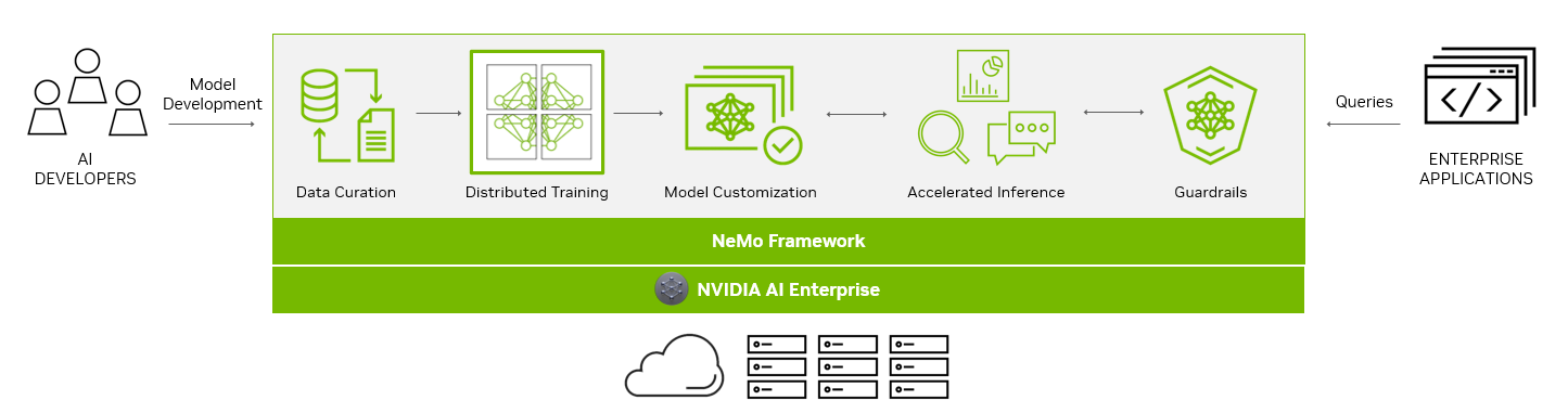
To aid you in creating LLMs, the NeMo framework provides powerful tools:
- Data curation
- Distributed training at scale
- Pretrained models for customization
- Accelerated inference
- Guardrails
Data curation
In the rapidly evolving landscape of AI, the demand for extensive datasets has become a critical factor in building robust LLMs.
The NeMo framework streamlines the often-complex process of data curation with NeMo Data Curator, which addresses the challenges of curating trillions of tokens in multilingual datasets. Through its scalability, this tool empowers you to effortlessly handle tasks like data download, text extraction, cleaning, filtering, and exact or fuzzy deduplication.
By harnessing the power of cutting-edge technologies, including Message-Passing Interface (MPI), Dask, and Redis Cluster, Data Curator can scale data-curation processes across thousands of compute cores, significantly reducing manual efforts and accelerating the development workflow.
One of the key benefits of Data Curator lies in its deduplication feature. By ensuring that LLMs are trained on unique documents, you can avoid redundant data and potentially achieve substantial cost savings during the pretraining phase. This not only streamlines the model development process but also optimizes AI investments for organizations, making AI development more accessible and cost-effective.
Data Curator comes packaged in the NeMo training container available through NGC.
Distributed training at scale
Training billion-parameter LLM models from scratch presents unique challenges of acceleration and scale. The process demands massive, distributed computing power, clusters of acceleration-based hardware and memory, reliable and scalable machine learning (ML) frameworks, and fault-tolerant systems.
At the heart of the NeMo framework lies the unification of distributed training and advanced parallelism. NeMo expertly uses GPU resources and memory across nodes, leading to groundbreaking efficiency gains. By dividing the model and training data, NeMo enables seamless multi-node and multi-GPU training, significantly reducing training time and enhancing overall productivity.
A standout feature of NeMo is its incorporation of various parallelism techniques:
- Data parallelism
- Tensor parallelism
- Pipeline parallelism
- Sequence parallelism
- Sparse attention reduction (SAR).
These techniques work in tandem to optimize the training process, thereby maximizing resource usage and bolstering performance.
NeMo also offers an array of precision options:
- FP32/TF32
- BF16
- FP8
Groundbreaking innovations like FlashAttention and Rotary Positional Embedding (RoPE) cater to long sequence-length tasks. Attention with Linear Biases (ALiBi), gradient and partial checkpointing, and the Distributed Adam Optimizer further elevate model performance and speed.
Pretrained models for customization
While some generative AI use cases require training from scratch, more and more organizations are using pretrained models to jump-start their effort when building customized LLMs.
One of the most significant benefits of pretrained models is the savings in time and resources. By skipping the data collection and cleaning phases required to pre-train the generic LLM, you can focus on fine-tuning models to their specific needs, accelerating the time to the final solution. Moreover, the burden of infrastructure setup and model training is greatly reduced, as pretrained models come with pre-existing knowledge, ready to be customized.
Thousands of open-source models are also available on hubs like GitHub, Hugging Face, and others, so you have choices when it comes to which model to start with. Accuracy is one of the more common measurements to evaluate pretrained models, but there are also other considerations:
- Size
- Cost to fine-tune
- Latency
- Memory constraints
- Commercial licensing options
With NeMo, you can now access a wide range of pretrained models, from NVIDIA and popular open-source repositories like Falcon AI, Llama-2, and MPT 7B.
NeMo models are optimized for inference, making them ideal for production use cases. With the ability to deploy these models in real-world applications, you can drive transformative outcomes and unlock the full potential of AI for your organizations.
Model customization
Customization of ML models is rapidly evolving to accommodate the unique needs of businesses and industries. The NeMo framework offers an array of techniques to refine generic, pretrained LLMs for specialized use cases. Through these diverse customization options, NeMo offers wide-ranging flexibility that is crucial in meeting varying business requirements.
Prompt engineering is an efficient customization method that makes it possible to use pretrained LLMs on many downstream tasks without needing to tune the pretrained models’ parameters. The goal of prompt engineering is to design and optimize prompts that are specific and clear enough to elicit the desired output from the model.
P-tuning and prompt tuning are parameter-efficient fine-tuning (PETF) techniques that use clever optimizations to selectively update only a few parameters of the LLM. As implemented in NeMo, new tasks can be added to a model without overwriting or disrupting previous tasks for which the model has already been tuned.
NeMo has optimized its p-tuning methods for use on multi-GPU and multi-node environments enabling accelerated training. NeMo p-tuning also supports an ‘early stop’ mechanism that identifies when a model has converged to the point when further training won’t improve accuracy much. It then stops the training job. This technique reduces the time and resources needed to customize models.
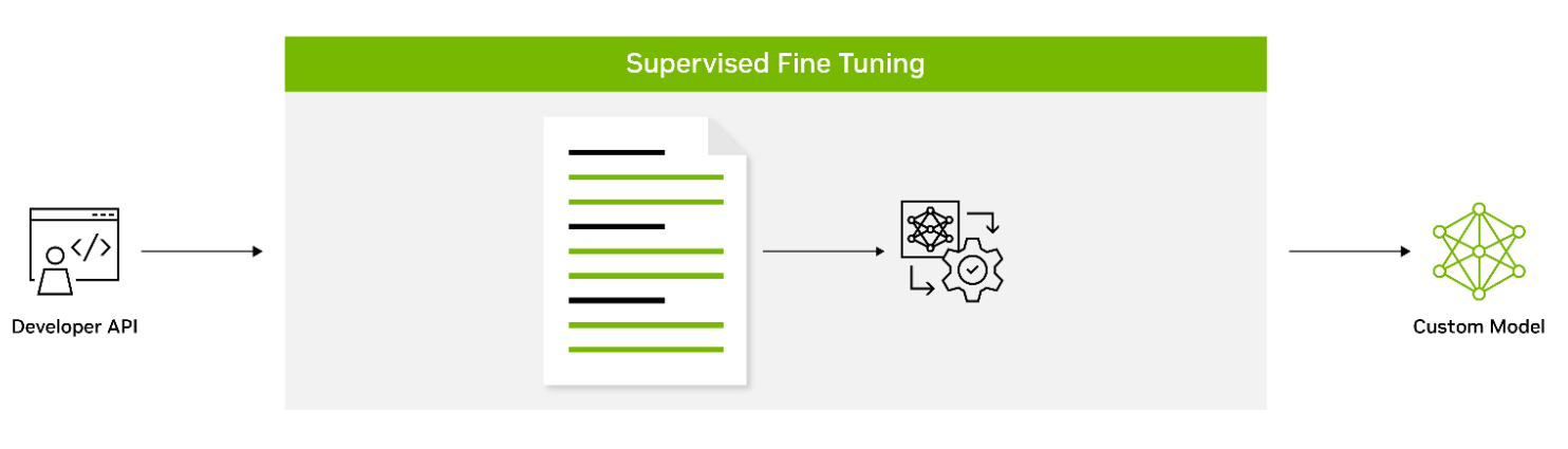
Supervised fine-tuning (SFT) involves fine-tuning a model’s parameters using labeled data. Also known as instruction tuning, this form of customization is typically conducted post-pretraining. It provides the advantage of using state-of-the-art models without the need for initial training, thus lowering computational costs and reducing data collection requirements.
Adapters introduce small feedforward layers in between the model’s core layers. These adapter layers are then fine-tuned for specific downstream tasks, providing a level of customization that is unique to the requirements of the task at hand.
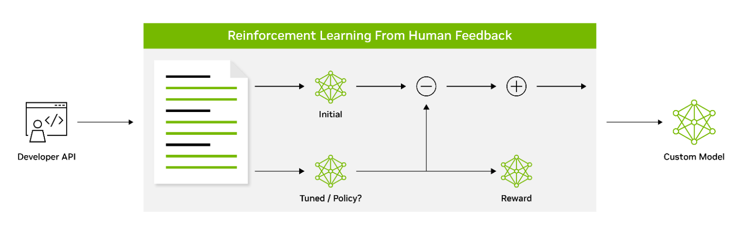
Reinforcement learning from human feedback (RLHF) employs a three-stage fine-tuning process. The model adapts its behavior based on feedback, encouraging a better alignment with human values and preferences. This makes RLHF a powerful tool for creating models that resonate with human users.
AliBi enables transformer models to process longer sequences at inference time than they were trained on. This is particularly useful in scenarios where the information to be processed is lengthy or complex.
NeMo Guardrails helps ensure that smart applications powered by LLMs are accurate, appropriate, on-topic, and secure. NeMo Guardrails is available as open source and includes all the code, examples, and documentation businesses need for adding safety to AI apps that generate text. NeMo Guardrails works with NeMo as well as all LLMs, including OpenAI’s ChatGPT.
Accelerated inference
Seamlessly integrating with NVIDIA Triton Inference Server, NeMo significantly accelerates the inference process, delivering exceptional accuracy, low latency, and high throughput. This integration facilitates secure and efficient deployments ranging from a single GPU to large-scale, multi-node GPUs, while adhering to stringent safety and security requirements.
NVIDIA Triton empowers NeMo to streamline and standardize generative AI inference. This enables teams to deploy, run, and scale trained ML or deep learning (DL) models from any framework on any GPU- or CPU-based infrastructure. This high level of flexibility provides you with the freedom to choose the most suitable framework for your AI research and data science projects without compromising production deployment flexibility.
Guardrails
As part of the NVIDIA AI Enterprise software suite, NeMo enables organizations to deploy production-ready generative AI with confidence. Organizations can take advantage of long-term branch support for up to 3 years, ensuring seamless operations and stability. Regular Common Vulnerabilities and Exposures (CVE) scans, security notifications, and timely patches enhance security, while API stability simplifies updates.
NVIDIA AI Enterprise support services are included with the purchase of the NVIDIA AI Enterprise software suite. We provide direct access to NVIDIA AI experts, defined service-level agreements, and control of upgrade and maintenance schedules with long-term support options.
Powering enterprise-grade generative AI
As part of NVIDIA AI Enterprise 4.0, NeMo offers seamless compatibility across multiple platforms, including the cloud, data centers, and now, NVIDIA RTX-powered workstations and PCs. This enables a true develop-once-and-deploy-anywhere experience, eliminates the complexities of integration, and maximizes operational efficiency.
NeMo has already gained significant traction among forward-thinking organizations looking to build custom LLMs. Writer and Korea Telecom have embraced NeMo, leveraging its capabilities to drive their AI-driven initiatives.
The unparalleled flexibility and support provided by NeMo opens a world of possibilities for businesses, enabling them to design, train, and deploy sophisticated LLM solutions tailored to their specific needs and industry verticals. By partnering with NVIDIA AI Enterprise and integrating NeMo into their workflows, your organizations can unlock new avenues of growth, derive valuable insights, and deliver cutting-edge AI-powered applications to customers, clients, and employees alike.
Get started with NVIDIA NeMo
NVIDIA NeMo has emerged as a game-changing solution, bridging the gap between the immense potential of generative AI and the practical realities faced by enterprises. A comprehensive platform for LLM development and deployment, NeMo empowers businesses to leverage AI technology efficiently and cost-effectively.
With these powerful capabilities, enterprises can integrate AI into their operations, streamlining processes, enhancing decision-making capabilities, and unlocking new avenues for growth and success.
Learn more about NVIDIA NeMo and how it helps enterprises build production-ready generative AI.