So my question is I have a variable which of type ops.Tensor. I need to convert this variable to a numpy variable. I tried different solutions online but in those cases the variable needs to be ops.EagerTensor to convert the variable into numpy object(. numpy (), tf.make_ndarray etc). Soo how can I convert my tensor object to eager tensor object or directly to numpy??
Create a compact desktop cluster with four NVIDIA Jetson Xavier NX modules to accelerate training and inference of AI and deep learning workflows.
Following in the footsteps of large-scale supercomputers like the NVIDIA DGX SuperPOD, this post guides you through the process of creating a small-scale cluster that fits on your desk. Below is the recommended hardware and software to complete this project. This small-scale cluster can be utilized to accelerate training and inference of artificial intelligence (AI) and deep learning (DL) workflows, including the use of containerized environments from sources such as the NVIDIA NGC Catalog.
While the Seeed Studio Jetson Mate, USB-C PD power supply, and USB-C cable are not required, they were used in this post and are highly recommended for a neat and compact desktop cluster solution.
Write the JetPack image to a microSD card and perform initial JetPack configuration steps:
The first iteration through this post is targeted toward the Slurm control node (slurm-control). After you have the first node configured, you can either choose to repeat each step for each module, or you can clone this first microSD card for the other modules; more detail on this later.
If you have already set the hostname in the initial JetPack setup, this step can be skipped.
[slurm-control]
sudo hostnamectl set-hostname slurm-control
sudo sed -i "s/127.0.1.1.*/127.0.1.1t`hostname`/" /etc/hosts
[compute-node]
Compute nodes should follow a particular naming convention to be easily addressable by Slurm. Use a consistent identifier followed by a sequentially incrementing number (for example, node1, node2, and so on). In this post, I suggest using nx1, nx2, and nx3 for the compute nodes. However, you can choose anything that follows a similar convention.
sudo hostnamectl set-hostname nx[1-3]
sudo sed -i "s/127.0.1.1.*/127.0.1.1t`hostname`/" /etc/hosts
Verify that the Munge encryption keys match from a compute node to slurm-control:
[compute-node]
munge -n | ssh slurm-control unmunge
Expected result: STATUS: Success (0)
Install Slurm (20.11.9):
cd ~
wget https://download.schedmd.com/slurm/slurm-20.11-latest.tar.bz2
tar -xjvf slurm-20.11-latest.tar.bz2
cd slurm-20.11.9
./configure --prefix=/usr/local
sudo make install -j6
Index the Slurm shared objects and copy the systemd service files:
For this step, you can follow the included commands and use the following configuration file for the cluster (recommended). To customize variables related to Slurm, use the configuration tool.
When replicating the configuration across the remaining nodes, label the JetsonNX modules with the assigned node name and/or the microSD cards. This helps prevent confusion later on when moving modules or cards around.
There are two different methods in which you can replicate your installation to the remaining modules: manual configuration or cloning slurm-control. Read over both methods and choose which method you prefer.
Manually configure the remaining nodes
Follow the “Enable and start the Slurm service daemon” section below for your current module, then repeat the entire processfor the remaining modules, skipping any steps tagged under [slurm-control]. When all modules are fully configured, install them into the Jetson Mate in their respective slots, as outlined in the “Install all Jetson Xavier NX modules into the enclosure” section.
Clone slurm-control installation for remaining nodes
To avoid repeating all installation steps for each node, clone the slurm-control node’s card as a base image and flash it onto all remaining cards. This requires a microSD-to-SD card adapter if you have only one multi-port card reader and want to do card-to-card cloning. Alternatively, creating an image file from the source slurm-control card onto the local machine and then flashing target cards is also an option.
Shut down the Jetson that you’ve been working with, remove the microSD card from the module, and insert it into the card reader.
If you’re performing a physical card to card clone (using Balena Etcher, dd, or any other utility that will do sector by sector writes), insert the blank target microSD into the SD card adapter, then insert it into the card reader.
Identify which card is which for the source (microSD) and destination (SD card) in the application that you’re using and start the cloning process.
If you are creating an image file, using a utility of your choice, create an image file from the slurm-control microSD card on the local machine, then remove that card and flash the remaining blank cards using that image.
After cloning is completed, insert a cloned card into a Jetson module and power on. Configure the node hostname for a compute node, then proceed to enable and start the Slurm service daemon. Repeat this process for all remaining card/module pairs.
Install all Jetson Xavier NX modules into the enclosure
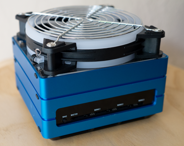
First power down any running modules, then remove them from their carriers. Install all Jetson modules into the Seeed Studio Jetson Mate, ensuring that the control node is placed in the primary slot labeled “MASTER”, and compute nodes 1-3 are placed in secondary slots labeled “WORKE 1, 2, and 3” respectively. Optional fan extension cables are available from the Jetson Mate kit for each module.
The video output on the enclosure is connected to the primary module slot, as is the vertical USB2 port, and USB3 port 1. All other USB ports are wired to the other modules according to their respective port numbers.
Figure 1. Fully assembled cluster inside of the SeeedStudio Jetson Mate
Troubleshooting
This section contains some helpful commands to assist in troubleshooting common networking and Slurm-related issues.
Test network configuration and connectivity
The following command should show eth0 in the routable state, with IP address information obtained from the DHCP server:
networkctl status
The command should respond with the local node’s hostname and .local as the domain (for example, slurm-control.local), along with DHCP assigned IP addresses:
host `hostname`
Choose a compute node hostname that is configured and online. It should respond similarly to the previous command. For example: host nx1 – nx1.local has address 192.168.0.1. This should also work for any other host that has an mDNS resolver daemon running on your LAN.
host [compute-node-hostname]
All cluster nodes should be pingable by all other nodes, and all local LAN IP addresses should be pingable as well, such as your router.
Test the external DNS name resolution and confirm that routing to the internet is functional:
ping www.nvidia.com
Check Slurm cluster status and node communication
The following command shows the current status of the cluster, including node states:
sinfo -lNe
If any nodes in the sinfo output show UNKNOWN or DOWN for their state, the following command signals to the specified nodes to change their state and become available for job scheduling ([ ] specifies a range of numbers following the hostname ‘nx’):
The following command runs hostname on all available compute nodes. Nodes should respond back with their corresponding hostname in your console.
srun -N3 hostname
Summary
You’ve now successfully built a multi-node Slurm cluster that fits on your desk. There’s a vast amount of benchmarks, projects, workloads, and containers that you can now run on your mini-cluster. Feel free to share your feedback on this post and, of course, anything that your new cluster is being used for.
Power on and enjoy Slurm!
For more information, see the following resources:
Special thanks to Robert Sohigian, a technical marketing engineer on our team, for all the guidance in creating this post, providing feedback on the clarity of instructions, and for being the lab rat in multiple runs of building this cluster. Your feedback was invaluable and made this post what it is!
Leading security, storage, and networking vendors are joining the DOCA and DPU community.
The DPU, or data processing unit, is a new class of programmable processors that specializes in moving data around the data center and now joins CPUs and GPUs as the third pillar of modern computing. NVIDIA DOCA is core to the NVIDIA Bluefield DPU offering because it provides ecosystem partners with an open platform to deliver the advanced networking, storage, and security services needed today.
DOCA unlocks data center innovation by enabling an open ecosystem and developer community to rapidly create applications and services on top of Bluefield DPUs, using industry-standard open APIs and frameworks.
Integral to our customers’ success, and our own, is the collaboration with our ecosystem partners. For more than 15 years, our ecosystem partners have harnessed the power of CUDA to develop the world’s most effective accelerated applications for a multitude of use cases.
The NVIDIA CUDA Toolkit provides everything that is needed to develop GPU-accelerated applications. Similarly, the NVIDIA DOCA Software Framework is an open SDK that enables you to rapidly create applications and services on top of Bluefield DPUs.
Where partners have achieved such success with NVIDIA GPUs and CUDA, we are emulating that formula with our DPU portfolio and DOCA. Moreover, we recognize that to deliver best-in-class solutions for customers, we need to partner with the world’s leading technology vendors. Proprietary applications have their place, but who better to provide world-class security, storage, and networking solutions, than the world’s leading vendors in those fields?
A meeting of the minds
During the last two years, our ecosystem partners have been delivering innovative solutions and services essential for digital transformation. The most turbulent period in recent history has forced us all to find new ways to collaborate and embrace technology at a rate never expected. Not only have we had to adapt as individuals, but organizations across the globe have been forced to re-think their day-to-day activities.
We work closely with our partners to define and create more DOCA libraries and services to address innovative use cases. More than ever, we’re witnessing a realignment between technology requirements in the data center and ever-changing business priorities. In turn, matching customers to ecosystem partners provides an opportunity to create customized technology solutions tuned to meet specific business objectives.
Today, NVIDIA is working with leading platform vendors and partners to integrate and expand DOCA support for commercial distributions on BlueField DPUs. Dozens of industry leaders, including VMWare, Red Hat, DDN, Aria Cybersecurity, and Juniper Networks, have started to integrate their solutions using the DPU/DOCA architecture. You’ll start to see more new applications in the coming year.
Earlier this year, Palo Alto Networks, a global cybersecurity leader developed the first next-generation firewall (NGFW) specifically designed to be accelerated by the BlueField DPU. This first-to-market, hardware-accelerated software NGFW is a prime example of how the BlueField DPU boosts performance and optimizes data center security coverage and efficiency.
Third-party developers can create and distribute DPU-accelerated applications with the DOCA SDK, which is fully integrated into the NGC catalog of containerized software. Such accelerated solutions will be wide-ranging, including advanced applications for infrastructure, storage, and security. It will be the key to unlocking data center innovation.
Try DOCA today
NVIDIA DOCA is the key to unlocking the potential of the NVIDIA BlueField DPU to offload, accelerate, and isolate data center workloads. With DOCA, you can program the data center infrastructure of tomorrow by creating software-defined, cloud-native, DPU-accelerated services with zero-trust protection to address the increasing performance and security demands of modern data centers.
Join us on July 20 for a webinar highlighting how using NVIDIA A100 GPUs can help map and location-based service providers speed up map creation and workflows, while reducing costs.
This post covers best practices for Vulkan clearing and presentation on NVIDIA GPUs. To get a high and consistent frame rate in your applications, see all Advanced API Performance tips.
This post covers best practices for Vulkan clearing and presenting on NVIDIA GPUs. To get a high and consistent frame rate in your applications, see all Advanced API Performance tips.
With the recent Vulkan 1.3 release, it’s timely to add some Vulkan-specific tips that are not necessarily explicitly covered by the other Advanced API Performance posts. In addition to introducing new Vulkan 1.3 core features, this post shares a set of good practices for clearing and presenting surfaces.
Vulkan 1.3 Core
Vulkan 1.3 brings improvements through extensions to key parts in the API. This section summarizes our recommendations for obtaining the best performance when working with a number of these new features.
Recommended
Skip framebuffer and render pass object setup by taking advantage of dynamic rendering.
Reduce the number of pipeline state objects with core support for dynamic states.
Simplify synchronization and avoid unnecessary image layout transitions by using the improved synchronization API
Clears
This section provides a guideline for achieving performance when invoking clear commands. This type of command clears a region within a color image or within the bound framebuffer attachments.
Use VK_ATTACHMENT_LOAD_OP_CLEAR to clear attachments at the beginning of a subpass instead of clear commands. This can allow the driver to skip loading unnecessary data.
Outside of a render pass instance, prefer the usage of vkCmdClearColorImage instead of a CS invocation to clear images. This path enables bandwidth optimizations.
If possible, batch clears to avoid interleaving single clears between dispatches.
Coordinate VkClearDepthStencilValue with the test function to achieve better depth testing performance:
0.5 ≤ depth value VK_COMPARE_OP_LESS_OR_EQUAL
0.0 ≤ depth value VK_COMPARE_OP_GREATER_OR_EQUAL
Not recommended
Specifying more than 30 unique clear values per application (or more than 15 on Turing) does not make the most of clear bandwidth optimizations.
“Clear shaders” should be avoided unless there is overlap of a compute clear with a neighboring dispatch.
Present
The following section offers insight into the preferred way of using the presentation modes supported by a surface in order to achieve good performance.
Recommended
Rely on VK_PRESENT_MODE_FIFO_KHR or VK_PRESENT_MODE_MAILBOX_KHR (for VSync on). Noteworthy aspects:
VK_PRESENT_MODE_FIFO_KHR is preferred as it does not drop frames and lacks tearing.
VK_PRESENT_MODE_MAILBOX_KHR may offer lower latency, but frames might be dropped.
VK_PRESENT_MODE_FIFO_RELAXED_KHR is compelling when your application only occasionally lags behind the refresh rate, allowing tearing so that it can “catch back up”.
Rely on VK_PRESENT_MODE_IMMEDIATE_KHR for VSync off.
On Windows systems, use the VK_EXT_full_screen_exclusive extension to bypass compositing.
Handle both out-of-date and suboptimal swapchains to re-create stale swapchains when windows resize, for example.
For latency-sensitive applications, use the Vulkan Reflex SDK to minimize latency by completing game engine work just-in-time for rendering.
With Nsight Systems, you can view Vulkan usage on a unified CPU-GPU timeline, investigate stutter, and track GPU cold spots to their CPU origins. Download Nsight Systems for free.
Acknowledgments
Thanks to Piers Daniell, Ivan Fedorov, Adam Moss, Ryan Prescott, Joshua Schnarr, Juha Sjöholm, and Márton Tamás for their feedback and contributions.
NVIDIA is helping push the limits of training AI generalist agents with a new open-sourced framework called MineDojo.
Using video games as a medium for training AI has become a popular method within the AI research community. These autonomous agents have had great success in Atari games, Starcraft, Dota, and Go. But while these advancements have been popular for AI research, the agents do not generalize beyond a very specific set of tasks, unlike humans that continuously learn from open-ended tasks.
Building an embodied agent that can attain high-level performance across a wide spectrum of tasks has been one of the greatest challenges facing the AI research community. In order to build a successful generalist agent, users need an environment that supports a multitude of tasks and goals, a large-scale database of multimodal knowledge, and a flexible and scalable agent architecture.
Enter Minecraft, the most played game in the world. With its flexible gameplay players can do a wide variety of actions. This ranges from building a medieval castle to exploring dangerous environments to gathering resources for building a Nether Portal to battle the Nether Dragon. This creative atmosphere is the perfect environment for an embodied agent to train.
Figure 1. The NVIDIA AI agent follows the prompts within the MineDojo framework
To take advantage of such an optimal training ground, NVIDIA researchers created MineDojo. MineDojo has built a massive framework that features a simulation suite with thousands of diverse open-ended tasks and an internet-scale knowledge base. Building an AI powerful enough to complete these tasks would not be possible without an expansive data library.
The mission of MineDojo is to promote research towards the goal of generally capable embodied agents. In order for the embodied agent to be successful, the environment needs to provide an almost infinite number of open-ended tasks and actions. This is done by giving the agent access to a large database of information to pull knowledge and then apply learnings. The training gained from the embodied agent needs to be scalable to convert the large-scale knowledge into actionable insights later on.
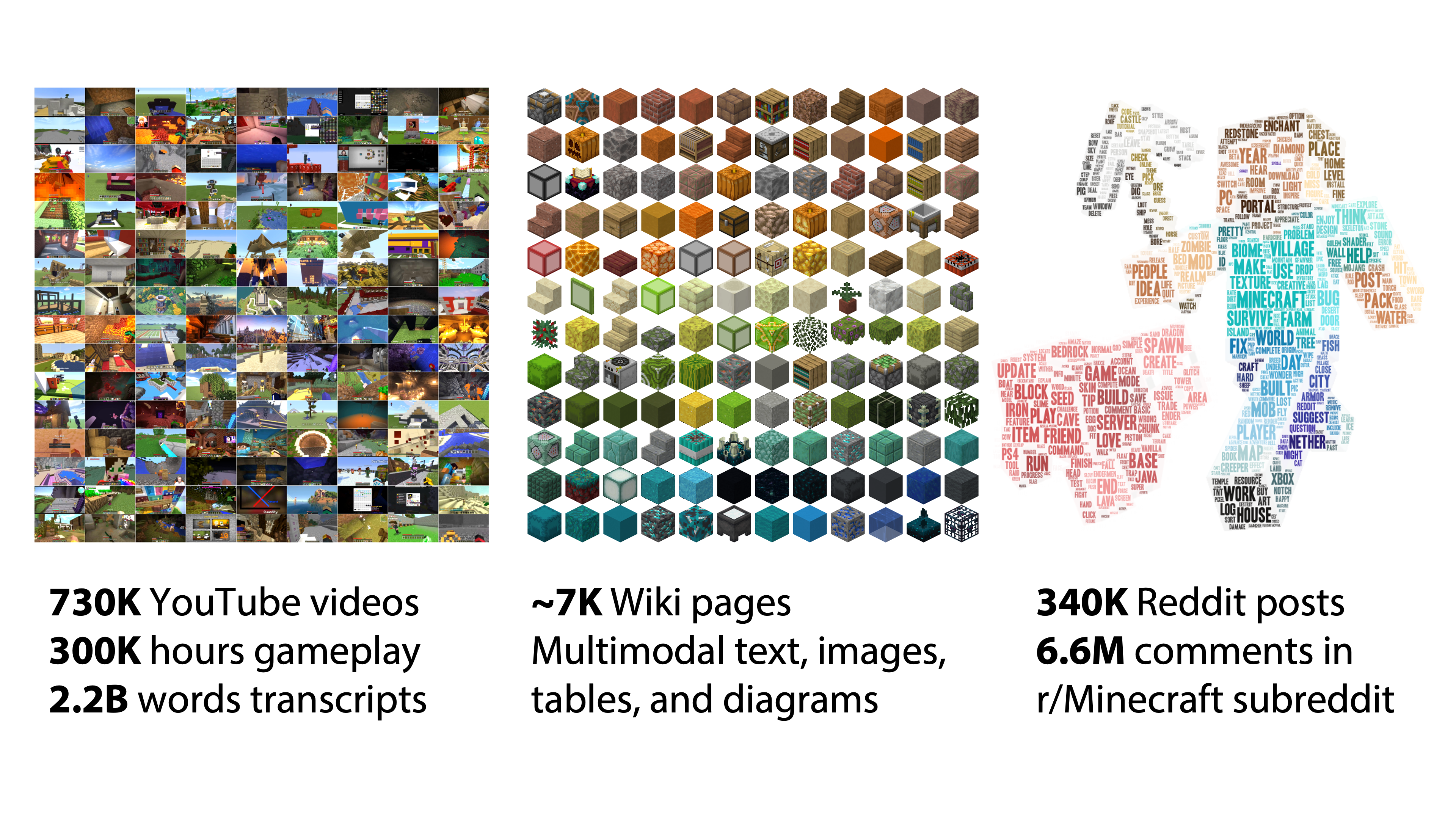
Figure 2. The MineDojo framework takes advantage of an Internet-scale database to train an AI agent
In MineDojo, the embodied agent has access to three internet-scale datasets. With 750,000 Minecraft YouTube videos—amounting to over 33 years of Minecraft videos—pulled into the database, over 2 million words were transcribed.
MineDojo also scraped over 6,000 web pages from the Minecraft Wiki, with over 2.2 million bounding boxes created for the visual elements of those pages). Also, millions of Reddit threads related to Minecraft and the variety of activities one can do within the game were captured. The questions included how to solve certain tasks and showcase achievements and creations in image and video formats, along with general tips and tricks.
Figure 3. Examples of content annotated and scraped from the internet for the MineDojo framework
MineDojo offers a set of simulator APIs that users can use to train their AI agents. It provides unified observation and action spaces to help facilitate the agent to adapt to new scenarios and multitask. Additionally, using the APIs users can take advantage of all three worlds within the Minecraft universe to expand on the number of tasks and actions the agent can do.
Within the simulator, MIneDojo splits the benchmarking tasks into two categories: programmatic tasks and creative tasks.
Programmatic tasks are well defined and can be easily evaluated, such as “surviving 3 days” or “obtain one unit of pumpkin in the forest.”
Creative tasks are much more open-ended, such as “build a beautiful beach house.” It is very difficult to define what qualifies as a beach house by an explicit set of rules. these tasks are to encourage the research community to develop more human-like and imaginative AI agents.
Figure 4. MineDojo currently provides benchmarks for thousands of creative and programmatic tasks
Natural language is a cornerstone of the MineDojo framework. It aids open-vocabulary understanding, provides grounding for image and video modalities, and serves as an intuitive interface to specify instructions. Combined with the latest speech recognition technology, it is possible in the near future to talk to an AI Agent as you would to a friend in multiplayer co-op mode.
For example: “plant a row of blue flowers in front of our house. Add some gold decorations to the door frame. Let’s go explore the cave next to the river,” could all be possible.
Proof of concept using MineCLIP
To help promote the project and provide a proof of concept, the MineDojo researchers have implemented a single language-prompted agent to complete several complex tasks within Minecraft, called MineCLIP. This novel agent learning algorithm takes advantage of the 33 years worth of Minecraft YouTube videos. However, it is good to point out that any agent can use any or all three sections of the Internet-scale database at the user’s discretion.
Figure 5. MineCLIP learns to associate video and text from the large amount of YouTube videos. The association score provides a reward signal to guide the agent to learn multiple tasks in parallel
MineCLIP as an embodied agent learns from the YouTube videos the concepts and actions of Minecraft without human hand labeling. YouTubers typically narrate what they are doing as they stream the gameplay video. MineCLIP is a large Transformer model that learns to associate a video clip and its corresponding English transcripts.
This association score can be provided as a reward signal to guide a reinforcement learning agent towards completing the task. For the example task, “shear a sheep to obtain wool,” MineCLIP gives a high reward to the agent if it approaches the sheep, but a low reward if the agent wanders aimlessly. It is even capable of multitasking within the game to complete a wide range of simple tasks.
Building generally capable embodied agents is a holy grail goal of AI research. MineDojo provides a benchmark of 1000s of tasks, an internet-scale rich knowledge base, and an innovative algorithm as a first step towards solving the grand challenge.
Stay posted to see what new models and techniques the research community comes up with next! Start using MineDojo today.
Hi all,
Hopefully this is no against any group rules, but I’m a DS master degree student coming from a CS bachelor, and I really love DeepLearning and all the magics that we can do solving optimization problems, even without NN involved.
I have a good preparation from the theoretical POV thanks to the university, and i’ve coded manually many optimization problem calculating gradient by hand, however I love the idea of autodiff that TF and PyTorch gives out of the box, and I’m really looking forward to learn TF from the ground up, however I really struggle to find material that does not lead in just stacking layers on a sequential model from Keras…
My aim is to be able to take an idea of (example) a layer, and code it using tensors and autodiff from TF, and not looking for online code that already solves that (or even maybe optimizers, since I’m pretty familiar to many other not already implemented in TF)
Do you have any online resource or book that you feel that is a good starting point? I usually learn hand on and reading Docs, however I feel like TF is better to learn it how it’s supposed to, to fully grasp everything that it can offers
In other words, I have a good theoretical preparation on ML/DL but I feel I’m lacking in a more practical aspect… so… how/where can I learn to use GradientTape and of those magic things (everything is accepted, online offline, paper digital, paid not paid)?
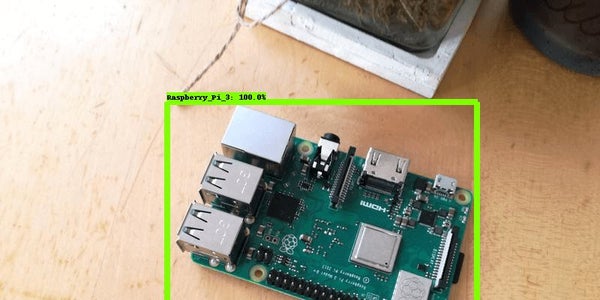
I am having an issue trying to make use of the tutorial below for Object Detection using tensor flow. I have tried to stick closely with the tutorial with changes only for my alternative labeled imageset.
When I attempt to run a python script to use the model with my webcam, I get the following error…
Traceback (most recent call last): File "detect_from_webcam.py", line 89, in <module> detection_model = load_model(args.model) File "detect_from_webcam.py", line 21, in load_model model = tf.saved_model.load(model_path) File "/usr/local/lib/python3.6/dist-packages/tensorflow/python/saved_model/load.py", line 864, in load result = load_internal(export_dir, tags, options)["root"] File "/usr/local/lib/python3.6/dist-packages/tensorflow/python/saved_model/load.py", line 903, in load_internal ckpt_options, options, filters) File "/usr/local/lib/python3.6/dist-packages/tensorflow/python/saved_model/load.py", line 165, in __init__ self._restore_checkpoint() File "/usr/local/lib/python3.6/dist-packages/tensorflow/python/saved_model/load.py", line 476, in _restore_checkpoint load_status = saver.restore(variables_path, self._checkpoint_options) File "/usr/local/lib/python3.6/dist-packages/tensorflow/python/training/tracking/util.py", line 1383, in restore checkpoint=checkpoint, proto_id=0).restore(self._graph_view.root) File "/usr/local/lib/python3.6/dist-packages/tensorflow/python/training/tracking/base.py", line 254, in restore restore_ops = trackable._restore_from_checkpoint_position(self) # pylint: disable=protected-access File "/usr/local/lib/python3.6/dist-packages/tensorflow/python/training/tracking/base.py", line 981, in _restore_from_checkpoint_position tensor_saveables, python_saveables)) File "/usr/local/lib/python3.6/dist-packages/tensorflow/python/training/tracking/util.py", line 352, in restore_saveables validated_saveables).restore(self.save_path_tensor, self.options) File "/usr/local/lib/python3.6/dist-packages/tensorflow/python/training/saving/functional_saver.py", line 339, in restore restore_ops = restore_fn() File "/usr/local/lib/python3.6/dist-packages/tensorflow/python/training/saving/functional_saver.py", line 323, in restore_fn restore_ops.update(saver.restore(file_prefix, options)) File "/usr/local/lib/python3.6/dist-packages/tensorflow/python/training/saving/functional_saver.py", line 116, in restore restored_tensors, restored_shapes=None) File "/usr/local/lib/python3.6/dist-packages/tensorflow/python/training/saving/saveable_object_util.py", line 132, in restore self.handle_op, self._var_shape, restored_tensor) File "/usr/local/lib/python3.6/dist-packages/tensorflow/python/ops/resource_variable_ops.py", line 309, in shape_safe_assign_variable_handle shape.assert_is_compatible_with(value_tensor.shape) File "/usr/local/lib/python3.6/dist-packages/tensorflow/python/framework/tensor_shape.py", line 1161, in assert_is_compatible_with raise ValueError("Shapes %s and %s are incompatible" % (self, other)) ValueError: Shapes (1, 1, 64, 108) and (1, 1, 64, 36) are incompatible
The primary issue seems to be the ValueError: Shapes (1, 1, 64, 108) and (1, 1, 64, 36) are incompatible reference. Unfortunately I am diving into Tensorflow Object detection headfirst without much background context. I am struggling to understand what is actually occurring with this error and what it means and where to even start looking for a resolution.
Any guidance at all would be exceedingly helpful.
Update:
I made a slight adjustment to my exporter_main_v2.py arguments which now results in the slightly different error… ValueError: Shapes (1, 1, 64, 54) and (1, 1, 64, 36) are incompatible.
Learn how NVIDIA Inception member Minerva CQ is using NVIDIA Riva to deliver faster, personalized experiences within a global EV charging and electric mobility company.
Posted by Dan Walker and Dan Liebling, Software Engineers, Google Research
People don’t write in the same way that they speak. Written language is controlled and deliberate, whereas transcripts of spontaneous speech (like interviews) are hard to read because speech is disorganized and less fluent. One aspect that makes speech transcripts particularly difficult to read is disfluency, which includes self-corrections, repetitions, and filled pauses (e.g., words like “umm”, and “you know”). Following is an example of a spoken sentence with disfluencies from the LDC CALLHOME corpus:
But that’s it’s not, it’s not, it’s, uh, it’s a word play on what you just said.
It takes some time to understand this sentence — the listener must filter out the extraneous words and resolve all of the nots. Removing the disfluencies makes the sentence much easier to read and understand:
But it’s a word play on what you just said.
While people generally don’t even notice disfluencies in day-to-day conversation, early foundational work in computational linguistics demonstrated how common they are. In 1994, using the Switchboard corpus, Elizabeh Shriberg demonstrated that there is a 50% probability for a sentence of 10–13 words to include a disfluency and that the probability increases with sentence length.
The proportion of sentences from the Switchboard dataset with at least one disfluency plotted against sentence length measured in non-disfluent (i.e., efficient) tokens in the sentence. The longer a sentence gets, the more likely it is to contain a disfluency.
In “Teaching BERT to Wait: Balancing Accuracy and Latency for Streaming Disfluency Detection”, we present research findings on how to “clean up” transcripts of spoken text. We create more readable transcripts and captions of human speech by finding and removing disfluencies in people’s speech. Using labeled data, we created machine learning (ML) algorithms that identify disfluencies in human speech. Once those are identified we can remove the extra words to make transcripts more readable. This also improves the performance of natural language processing (NLP) algorithms that work on transcripts of human speech. Our work puts special priority on ensuring that these models are able to run on mobile devices so that we can protect user privacy and preserve performance in scenarios with low connectivity.
Base Model Overview At the core of our base model is a pre-trained BERTBASE encoder with 108.9 million parameters. We use the standard per-token classifier configuration, with a binary classification head being fed by the sequence encodings for each token.
Illustration of how tokens in text become numerical embeddings, which then lead to output labels.
<!–
Illustration of how tokens in text become numerical embeddings, which then lead to output labels.
–>
We refined the BERT encoder by continuing the pretraining on the comments from the Pushrift Reddit dataset from 2019. Reddit comments are not speech data, but are more informal and conversational than the wiki and book data. This trains the encoder to better understand informal language, but may run the risk of internalizing some of the biases inherent in the data. For our particular use case, however, the model only captures the syntax or overall form of the text, not its content, which avoids potential issues related to semantic-level biases in the data.
We fine-tune our model for disfluency classification on hand-labeled corpora, such as the Switchboard corpus mentioned above. Hyperparameters (batch size, learning rate, number of training epochs, etc.) were optimized using Vizier.
We also produce a range of “small” models for use on mobile devices using a knowledge distillation technique known as “self training”. Our best small model is based on the Small-vocab BERT variant with 3.1 million parameters. This smaller model achieves comparable results to our baseline at 1% the size (in MiB). You can read more about how we achieved this model miniaturization in our 2021 Interspeech paper.
Streaming Some of the latest use cases for automatic speech transcription include automated live captioning, such as produced by the Android “Live Captions” feature, which automatically transcribes spoken language in audio being played on the device. For disfluency removal to be of use in improving the readability of the captions in this setting, then it must happen quickly and in a stable manner. That is, the model should not change its past predictions as it sees new words in the transcript.
We call this live token-by-token processing streaming. Accurate streaming is difficult because of temporal dependencies; most disfluencies are only recognizable later. For example, a repetition does not actually become a repetition until the second time the word or phrase is said.
To investigate whether our disfluency detection model is effective in streaming applications, we split the utterances in our training set into prefix segments, where only the first N tokens of the utterance were provided at training time, for all values of N up to the full length of the utterance. We evaluated the model simulating a stream of spoken text by feeding prefixes to the models and measuring the performance with several metrics that capture model accuracy, stability, and latency including streaming F1, time to detection (TTD), edit overhead (EO), and average wait time (AWT). We experimented with look-ahead windows of either one or two tokens, allowing the model to “peek” ahead at additional tokens for which the model is not required to produce a prediction. In essence, we’re asking the model to “wait” for one or two more tokens of evidence before making a decision.
While adding this fixed look-ahead did improve the stability and streaming F1 scores in many contexts, we found that in some cases the label was already clear even without looking ahead to the next token and the model did not necessarily benefit from waiting. Other times, waiting for just one extra token was sufficient. We hypothesized that the model itself could learn when it should wait for more context. Our solution was a modified model architecture that includes a “wait” classification head that decides when the model has seen enough evidence to trust the disfluency classification head.
Diagram showing how the model labels input tokens as they arrive. The BERT embedding layers feed into two separate classification heads, which are combined for the output.
<!–
Diagram showing how the model labels input tokens as they arrive. The BERT embedding layers feed into two separate classification heads, which are combined for the output.
–>
We constructed a training loss function that is a weighted sum of three factors:
The traditional cross-entropy loss for the disfluency classification head
A cross-entropy term that only considers up to the first token with a “wait” classification
A latency penalty that discourages the model from waiting too long to make a prediction
We evaluated this streaming model as well as the standard baseline with no look-ahead and with both 1- and 2-token look-ahead values:
Graph of the streaming F1 score versus the average wait time in tokens. Three data points indicate F1 scores above 0.82 across multiple wait times. The proposed streaming model achieves near top performance with much shorter wait times than the fixed look ahead models.
The streaming model achieved a better streaming F1 score than both a standard baseline with no look ahead and a model with a look ahead of 1. It performed nearly as well as the variant with fixed look ahead of 2, but with much less waiting. On average the model waited for only 0.21 tokens of context.
Internationalization Our best outcomes so far have been with English transcripts. This is mostly due to resourcing issues: while there are a number of relatively large labeled conversational datasets that include disfluencies in English, other languages often have very few such datasets available. So, in order to make disfluency detection models available outside English a method is needed to build models in a way that does not require finding and labeling hundreds of thousands of utterances in each target language. A promising solution is to leverage multi-language versions of BERT to transfer what a model has learned about English disfluencies to other languages in order to achieve similar performance with much less data. This is an area of active research, but we do have some promising results to outline here.
As a first effort to validate this approach, we added labels to about 10,000 lines of dialogue from the German CALLHOME dataset. We then started with the Geotrend English and German Bilingual BERT model (extracted from Multilingual BERT) and fine-tuned it with approximately 77,000 disfluency-labeled English Switchboard examples and 1.3 million examples of self-labeled transcripts from the Fisher Corpus. Then, we did further fine tuning with about 7,500 in-house–labeled examples from the German CALLHOME dataset.
Diagram illustrating the flow of labeled data and self-trained output in our best multilingual training setup. By training on both English and German data we are able to improve performance via transfer learning.
Our results indicate that fine-tuning on a large English corpus can produce acceptable precision using zero-shot transfer to similar languages like German, but at least a modest amount of German labels were needed to improve recall from less than 60% to greater than 80%. Two-stage fine-tuning of an English-German bilingual model produced the highest precision and overall F1 score.
Approach
Precision
Recall
F1
German BERTBASE model fine-tuned on 7,300 human-labeled German CALLHOME examples
89.1%
81.3%
85.0
Same as above but with additional 7,500 self-labeled German CALLHOME examples
91.5%
83.3%
87.2
English/German Bilingual BERTbase model fine-tuned on English Switchboard+Fisher, evaluated on German CALLHOME (zero-shot language transfer)
87.2%
59.1%
70.4
Same as above but subsequently fine-tuned with 14,800 German CALLHOME (human- and self-labeled) examples
95.5%
82.6%
88.6
Conclusion Cleaning up disfluencies from transcripts can improve not just their readability for people, but also the performance of other models that consume transcripts. We demonstrate effective methods for identifying disfluencies and expand our disfluency model to resource-constrained environments, new languages, and more interactive use cases.
Acknowledgements Thank you to Vicky Zayats, Johann Rocholl, Angelica Chen, Noah Murad, Dirk Padfield, and Preeti Mohan for writing the code, running the experiments, and composing the papers discussed here. Wealso thank our technical product manager Aaron Schneider, Bobby Tran from the Cerebra Data Ops team, and Chetan Gupta from Speech Data Ops for their support obtaining additional data labels.

 Create a compact desktop cluster with four NVIDIA Jetson Xavier NX modules to accelerate training and inference of AI and deep learning workflows.
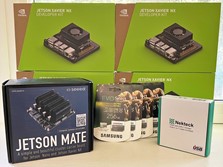
") Leading security, storage, and networking vendors are joining the DOCA and DPU community.
Leading security, storage, and networking vendors are joining the DOCA and DPU community.  Join us on July 20 for a webinar highlighting how using NVIDIA A100 GPUs can help map and location-based service providers speed up map creation and workflows, while reducing costs.
  This post covers best practices for Vulkan clearing and presentation on NVIDIA GPUs. To get a high and consistent frame rate in your applications, see all Advanced API Performance tips.
 NVIDIA is helping push the limits of training AI generalist agents with a new open-sourced framework called MineDojo.
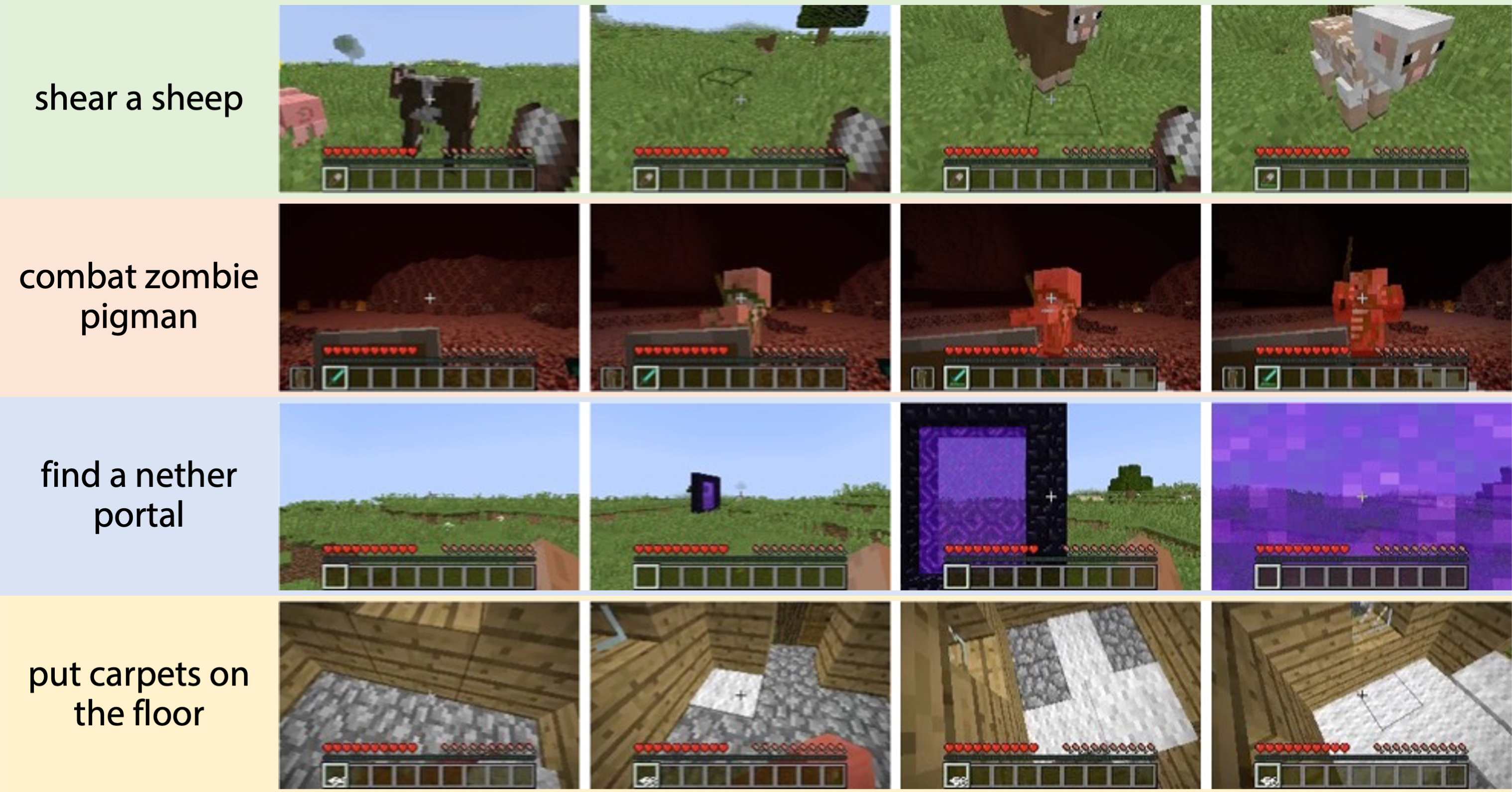

 Learn how NVIDIA Inception member Minerva CQ is using NVIDIA Riva to deliver faster, personalized experiences within a global EV charging and electric mobility company.
.png)


