The 15 accepted papers and posters from NVIDIA range from simulating dynamic driving environments, to powering neural architecture search for medical imaging.
Researchers, developers, and engineers worldwide are gathering virtually this year for the annual Conference on Computer Vision and Pattern Recognition (CVPR) from June 19th to June 25th. Throughout the week, NVIDIA Research will present their recent computer vision-related projects via presentations and interactive Q&As.
The nearly 30 accepted papers from NVIDIA range from simulating dynamic driving environments, to powering neural architecture search for medical imaging.
DriveGAN is a fully differentiable simulator, it further allows for re-simulation of a given video sequence, offering an agent to drive through a recorded scene again, possibly taking different actions.
The talk will be live on Tuesday, June 22, 2021 at 10:00pm EST
From the abstract: In this work, we focus on three important aspects of NAS in 3D medical image segmentation: flexible multi-path network topology, high search efficiency, and budgeted GPU memory usage. Our method achieves the state-of-the-art performance and the top ranking on the MSD challenge leaderboard.
The talk will be live on Tuesday, June 22, 2021 at 10:00 pm EST
To view the complete list of NVIDIA Research accepted papers, workshop and tutorials, demos, and to explore job opportunities at NVIDIA, visit the NVIDIA at CVPR 2021 website.
Nithya Sambasivan, Research Scientist, Google Research
Data is a foundational aspect of machine learning (ML) that can impact performance, fairness, robustness, and scalability of ML systems. Paradoxically, while building ML models is often highly prioritized, the work related to data itself is often the least prioritized aspect. This data work can require multiple roles (such as data collectors, annotators, and ML developers) and often involves multiple teams (such as database, legal, or licensing teams) to power a data infrastructure, which adds complexity to any data-related project. As such, the field of human-computer interaction (HCI), which is focused on making technology useful and usable for people, can help both to identify potential issues and to assess the impact on models when data-related work is not prioritized.
In “‘Everyone wants to do the model work, not the data work’: Data Cascades in High-Stakes AI”, published at the 2021 ACM CHI Conference, we study and validate downstream effects from data issues that result in technical debt over time (defined as “data cascades”). Specifically, we illustrate the phenomenon of data cascades with the data practices and challenges of ML practitioners across the globe working in important ML domains, such as cancer detection, landslide detection, loan allocation and more — domains where ML systems have enabled progress, but also where there is opportunity to improve by addressing data cascades. This work is the first that we know of to formalize, measure, and discuss data cascades in ML as applied to real-world projects. We further discuss the opportunity presented by a collective re-imagining of ML data as a high priority, including rewarding ML data work and workers, recognizing the scientific empiricism in ML data research, improving the visibility of data pipelines, and improving data equity around the world.
Origins of Data Cascades We observe that data cascades often originate early in the lifecycle of an ML system, at the stage of data definition and collection. Cascades also tend to be complex and opaque in diagnosis and manifestation, so there are often no clear indicators, tools, or metrics to detect and measure their effects. Because of this, small data-related obstacles can grow into larger and more complex challenges that affect how a model is developed and deployed. Challenges from data cascades include the need to perform costly system-level changes much later in the development process, or the decrease in users’ trust due to model mis-predictions that result from data issues. Nevertheless and encouragingly, we also observe that such data cascades can be avoided through early interventions in ML development.
Different color arrows indicate different types of data cascades, which typically originate upstream, compound over the ML development process, and manifest downstream.
Examples of Data Cascades One of the most common causes of data cascades is when models that are trained on noise-free datasets are deployed in the often-noisy real world. For example, a common type of data cascade originates from model drifts, which occur when target and independent variables deviate, resulting in less accurate models. Drifts are more common when models closely interact with new digital environments — including high-stakes domains, such as air quality sensing, ocean sensing, and ultrasound scanning — because there are no pre-existing and/or curated datasets. Such drifts can lead to more factors that further decrease a model’s performance (e.g., related to hardware, environmental, and human knowledge). For example, to ensure good model performance, data is often collected in controlled, in-house environments. But in the live systems of new digital environments with resource constraints, it is more common for data to be collected with physical artefacts such as fingerprints, shadows, dust, improper lighting, and pen markings, which can add noise that affects model performance. In other cases, environmental factors such as rain and wind can unexpectedly move image sensors in deployment, which also trigger cascades. As one of the model developers we interviewed reported, even a small drop of oil or water can affect data that could be used to train a cancer prediction model, therefore affecting the model’s performance. Because drifts are often caused by the noise in real-world environments, they also take the longest — up to 2-3 years — to manifest, almost always in production.
Another common type of data cascade can occur when ML practitioners are tasked with managing data in domains in which they have limited expertise. For instance, certain kinds of information, such as identifying poaching locations or data collected during underwater exploration, rely on expertise in the biological sciences, social sciences, and community context. However, some developers in our study described having to take a range of data-related actions that surpassed their domain expertise — e.g., discarding data, correcting values, merging data, or restarting data collection — leading to data cascades that limited model performance. The practice of relying on technical expertise more than domain expertise (e.g., by engaging with domain experts) is what appeared to set off these cascades.
Two other cascades observed in this paper resulted from conflicting incentives and organizational practices between data collectors, ML developers, and other partners — for example, one cascade was caused by poor dataset documentation. While work related to data requires careful coordination across multiple teams, this is especially challenging when stakeholders are not aligned on priorities or workflows.
How to Address Data Cascades Addressing data cascades requires a multi-part, systemic approach in ML research and practice:
Develop and communicate the concept of goodness of the data that an ML system starts with, similar to how we think about goodness of fit with models. This includes developing standardized metrics and frequently using those metrics to measure data aspects like phenomenological fidelity (how accurately and comprehensively does the data represent the phenomena) and validity (how well the data explains things related to the phenomena captured by the data), similar to how we have developed good metrics to measure model performance, like F1-scores.
Innovate on incentives to recognize work on data, such as welcoming empiricism on data in conference tracks, rewarding dataset maintenance, or rewarding employees for their work on data (collection, labelling, cleaning, or maintenance) in organizations.
Data work often requires coordination across multiple roles and multiple teams, but this is quite limited currently (partly, but not wholly, because of the previously stated factors). Our research points to the value of fostering greater collaboration, transparency, and fairer distribution of benefits between data collectors, domain experts, and ML developers, especially with ML systems that rely on collecting or labelling niche datasets.
Finally, our research across multiple countries indicates that data scarcity is pronounced in lower-income countries, where ML developers face the additional problem of defining and hand-curating new datasets, which makes it difficult to even start developing ML systems. It is important to enable open dataset banks, create data policies, and foster ML literacy of policy makers and civil society to address the current data inequalities globally.
Conclusion In this work we both provide empirical evidence and formalize the concept of data cascades in ML systems. We hope to create an awareness of the potential value that could come from incentivising data excellence. We also hope to introduce an under-explored but significant new research agenda for HCI. Our research on data cascades has led to evidence-backed, state-of-the-art guidelines for data collection and evaluation in the revised PAIR Guidebook, aimed at ML developers and designers.
Acknowledgements This paper was written in collaboration with Shivani Kapania, Hannah Highfill, Diana Akrong, Praveen Paritosh and Lora Aroyo. We thank our study participants, and Sures Kumar Thoddu Srinivasan, Jose M. Faleiro, Kristen Olson, Biswajeet Malik, Siddhant Agarwal, Manish Gupta, Aneidi Udo-Obong, Divy Thakkar, Di Dang, and Solomon Awosupin.
The Clara AGX SDK runs on the NVIDIA Jetson and Clara AGX platform and provides developers with capabilities to build end-to-end streaming workflows for medical imaging.
NVIDIA Clara AGX SDK 3.0 is available today! The Clara AGX SDK runs on the NVIDIA Jetson and Clara AGX platform and provides developers with capabilities to build end-to-end streaming workflows for medical imaging. The focus of this release is to provide added support for NGC containers, including TensorFlow and PyTorch frameworks, a new ultrasound application, and updated Transfer Learning Toolkit scripts.
NVIDIA Clara AGX SDK
There is now support for the leading deep learning framework containers, including TensorFlow 1, TensorFlow 2, and PyTorch, as well as the Triton Inference Server. These containers can help you quickly get started using the Clara AGX Development Kit, NVIDIA’s GPU super-charged development platform for AI medical devices and edge-based inferencing. We’ve also released three new application containers along with the SDK, available on NGC. These application containers include:
Metagenomics application
US4US Ultrasound application and sample code
Dermatology Melanoma detection
Clara AGX SDK has also been updated to the latest Transfer Learning Toolkit (TLT) 3.0 release. Developers can now use TLT 3.0 out-of-the-box and includes compatibility with DeepStream SDK for real-time, low latency, high-resolution image AI deployments.
Download Clara AGX SDK 3.0 through the Clara AGX Developer Site. An NVIDIA Developer Program account is needed to access the SDK. You can also find all of our containers through NGC.
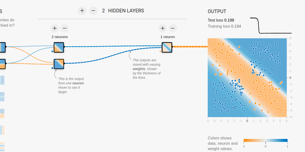
Hi guys, I’m trying to reproduce this mlp in tf (constraining it to have only one hidden layer with 2 units). However, like in playground tf, many times do not converge to global maxima. I think is due to weight initialization, tried xavier and he initializations but no success. The following piece of code is the model in tf keras.
model = tf.keras.models.Sequential([ Dense(units=2, activation='sigmoid', input_shape=(2,)), Dense(units=1, activation='sigmoid')
All the threads I’ve read online regarding utilizing multiple cores in python requires multiprocessing. By default python can only bye running on one core (and one on thread, because of the GIL).
On the other hand, I often read that tensorflow by default uses multiple cores. How can this work if python itself is limited to one core?
NVIDIA Train, Adapt, and Optimize (TAO) is an AI model adaptation platform that simplifies and accelerates the creation of enterprise AI applications.
Building a state-of-the-art deep learning model is a complex and time-consuming process. To achieve this, large datasets collected for the model must be of high quality. Once the data is collected, it must be prepared and then trained, and optimized over several iterations. This is not always an option for many enterprises looking to bring their AI applications to market faster while reducing operational costs.
NVIDIA TAO is being developed to address these challenges. NVIDIA Train, Adapt, and Optimize (TAO) is an AI model adaptation platform that simplifies and accelerates the creation of enterprise AI applications. By fine-tuning state-of-the-art pre-trained models created by NVIDIA experts with custom data through a UI-based, guided workflow, you can produce highly accurate computer vision, speech, and language understanding models in hours rather than months, eliminating the need for large training runs and deep AI expertise.
Registration for the Early Access Program is now open. Later this year we will begin accepting applicants into the program which will provide you with an exclusive opportunity to collaborate with the NVIDIA product team to help shape TAO.
Key Highlights of the Early Access Program:
Access to state-of-the-art accurate pre-trained models that can be customized for your use case
Access to compute infrastructure
Hands-on support to help you navigate through the entire process
Simulations are pervasive in every domain of science and engineering, but they are often constrained by large computational times, limited compute resources, tedious manual setup efforts, and the need for technical expertise. NVIDIA SimNet is a simulation toolkit that addresses these challenges with a combination of AI and physics. A success story of SimNet’s application … Continued
Simulations are pervasive in every domain of science and engineering, but they are often constrained by large computational times, limited compute resources, tedious manual setup efforts, and the need for technical expertise. NVIDIA SimNet is a simulation toolkit that addresses these challenges with a combination of AI and physics.
A success story of SimNet’s application today is in modeling the flow and transport in porous media. This effort was led by Cedric Frances, a PhD student at Stanford University.
Use case study
Cedric is researching the applicability and limitations of mesh-free reservoir simulations using physics-informed neural networks (PINNs). He’s keenly interested in the flow and transport problem in porous media (conservation of mass and Darcy flow). Cedric’s application is a Python-based reservoir simulator, which computes the pressure and concentrations of various fluids in a porous media and enables predictions that typically affect large, industrial energy projects. This includes the production of hydrocarbons, storage of carbon dioxide, water disposal, air storage, waste management, and so on.
Researchers previously tried to use the PINNs approach to capture the solution of a hyperbolic problem with nonconvex flux term (Riemann problem) in a forward setting with no data other than initial and boundary conditions. Unfortunately, these attempts were unsuccessful.
Before trying out SimNet, Cedric developed his own implementations of PINNs using Python and deep learning frameworks such as TensorFlow and Keras. He used various architectures of networks, such as residual, GAN, periodic activation, CNN, PDE-Net, and so on. However, it was difficult to implement all of them to find which one worked best or worked at all. The emergence of open-source code on GitHub made it easy to test these implementations out. The high overhead involved in every new implementation, such as environment setup, hardware configuration, modification of code to test his own problem, and so on, was not efficient.
Cedric wanted to have a good, unified framework maintained by a team of professional software developers to solve problems that allowed him to focus on the physics of the problem and extensively test the methods that have been recently published. His search for such a framework ended when he stumbled upon SimNet.
Cedric downloaded SimNet and started using fully connected networks with tanh activation functions and spatial weighing of the loss function. He discovered that SimNet’s general-purpose framework with multiple architectures and well-documented examples served as a good starting point. Its ability to emulate solutions with sharp shocks, introduce new dynamic constraints such as entropy and velocity saved him weeks of development. More importantly, it provided a quick turnaround on testing methods to determine their usefulness.
The problem presented here is that of incompressible, immiscible displacement of two phases in a porous medium. This is also referred to as transport problem and has been delineated in various forms over the years. It has been applied to the displacement of oil by water for waterflood problems in reservoir for over half a century. More recently, it’s been applied to the displacement of brine by CO2 in carbon sequestration applications. For more information, see Mechanism of Fluid Displacement in Sands and Theory of Gas Injection Processes.
Assume that a wetting phase (w) is displacing a nonwetting phase (n). Wettability is the preference of a fluid to be in contact with a solid surrounded by another fluid; for example, water is wetting on most surfaces compared to air. Conservation of mass applies to both phases. For the wetting phase:
(1)
In this formula, is the porosity, is the saturation (or concentration) of that wetting phase, and is the saturation of the nonwetting. The flow rate of the wetting phase can be written as follows:
(2)
In this formula, is the absolute permeability that quantifies the propensity of a material to allow liquid or gas to flow through it. is the wetting phase relative permeability that is function of the saturation and characterizes the effective permeability of a given phase in the presence or absence of it. A phase preferentially flows through a path where it is already present. Think of a drop of water dripping down from a window and following existing trails.
You can formulate the phase flux of the wetting phase as a function of the total flux using a simple homogenization rule:
(3)
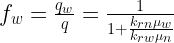
You can rewrite this equation as a function of the total flux. This gives rise to the fractional flow:
(4)
The conservation equation can now be written:
(5)
For a one-dimensional case where you assume that the total flux is equal to one pore volume injected per time step (), you can obtain the equation:
(6)
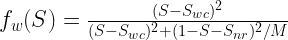
In this formula, the fractional flow is a nonlinear equation defined as follows:
(7)
In this formula, and are the residual (irreducible) saturations for the wetting and nonwettings resulting from trapping mechanisms and is the endpoint mobility ratio defined as the ratio of endpoint-relative permeability and viscosity of both phases. We used the Corey and Brooks relative permeability relationship. For more information, see Hydraulic Properties of Porous Media.
The partial differential equation solved here is a hyperbolic of order 1 and the fractional flow term is nonconvex. It belongs to the class of Riemann conservation problem that is typically solved using finite volume methods. For more information, see Hyperbolic systems of conservation laws and the mathematical theory of shock waves.
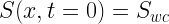
With uniform Dirichlet boundary conditions:
(8)
(9)
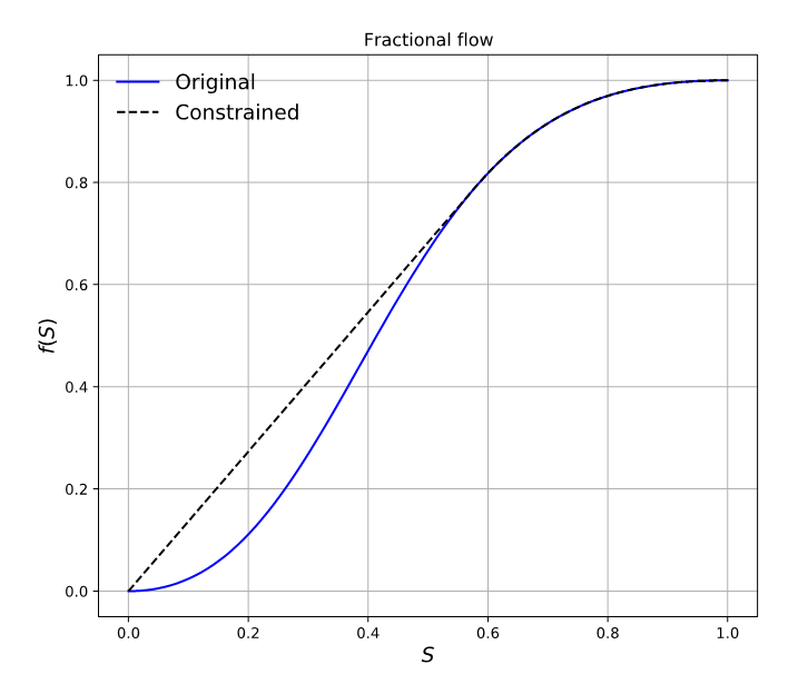
You can apply the method of characteristics (MOC) to build an analytical solution to this equation. For the MOC or any finite volume method to be conservative, you must modify the fractional flow term as shown in Figure 1.
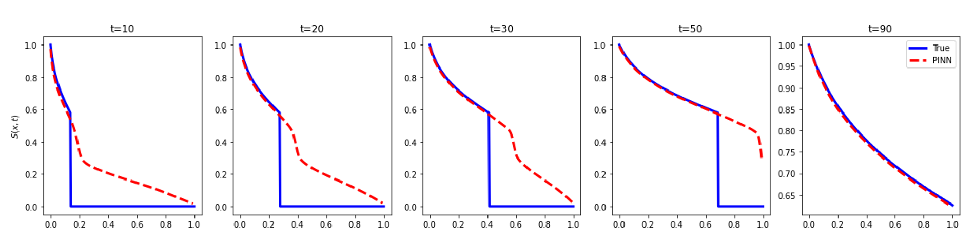
Until now, no other known method solved such a problem using a sampling method, so this remained an open question. A previous attempt by Fuks and Tchelepi concluded that physics-informed approaches were not suitable for the problem described (Figure 2).
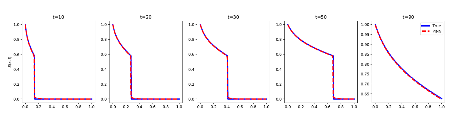
Figure 3. Results of saturation inference using PINN (dashed red) vs MOC (blue) with velocity constraint and entropy condition. The convex hull of the fractional flow curve is used to model the displacement. Source:Physics Informed Deep Learning for Flow and Transport in Porous Media
Important theoretical milestones are now being reached on simple yet challenging 1D examples. Cedric plans on expanding his study to larger dimensions (2D and 3D), where the scalability of the code and the easy deployment on larger arrays will be put to the test. He expects to encounter similar issues and is looking forward to the gain provided by SimNet going from 2D to 3D, for example.
Cedric elaborated on his experience with SimNet. “SimNet’s clear APIs, clean and easily navigable code, environment and hardware configurations well handled with Docker containers, scalability, ease of deployment and the competent support team made it easy to adopt and has provided some very promising results. This has been great so far and we look forward to using SimNet on problems with much larger dimensions.”
Daniel Ho, Software Engineer, The Everyday Robot Project and Kanishka Rao, Staff Software Engineer, Robotics at Google
Reinforcement and imitation learning methods in robotics research can enable autonomous environmental navigation and efficient object manipulation, which in turn opens up a breadth of useful real-life applications. Previous work has demonstrated how robots that learn end-to-end using deep neural networks can reliably and safely interact with the unstructured world around us by comprehending camera observations to take actions and solve tasks. However, while end-to-end learning methods can generalize and scale for complicated robot manipulation tasks, they require hundreds of thousands real world robot training episodes, which can be difficult to obtain. One can attempt to alleviate this constraint by using a simulation of the environment that allows virtual robots to learn more quickly and at scale, but the simulations’ inability to exactly match the real world presents a challenge c ommonly referred to as the sim-to-real gap. One important source of the gap comes from discrepancies between the images rendered in simulation and the real robot camera observations, which then causes the robot to perform poorly in the real world.
To-date, work on bridging this gap has employed a technique called pixel-level domain adaptation, which translates synthetic images to realistic ones at the pixel level. One example of this technique is GraspGAN, which employs a generative adversarial network (GAN), a framework that has been very effective at image generation, to model this transformation between simulated and real images given datasets of each domain. These pseudo-real images correct some sim-to-real gap, so policies learned with simulation execute more successfully on real robots. A limitation for their use in sim-to-real transfer, however, is that because GANs translate images at the pixel-level, multi-pixel features or structures that are necessary for robot task learning may be arbitrarily modified or even removed.
To address the above limitation, and in collaboration with the Everyday Robot Project at X, we introduce two works, RL-CycleGAN and RetinaGAN, that train GANs with robot-specific consistencies — so that they do not arbitrarily modify visual features that are specifically necessary for robot task learning — and thus bridge the visual discrepancy between sim and real. We demonstrate how these consistencies preserve features critical to policy learning, eliminating the need for hand-engineered, task-specific tuning, which in turn allows for this sim-to-real methodology to work flexibly across tasks, domains, and learning algorithms. With RL-CycleGAN, we describe our sim-to-real transfer methodology and demonstrate state-of-the-art performance on real world grasping tasks trained with RL. With RetinaGAN, we extend our approach to include imitation learning with a door opening task.
RL-CycleGAN In “RL-CycleGAN: Reinforcement Learning Aware Simulation-To-Real”, we leverage a variation of CycleGAN for sim-to-real adaptation by ensuring consistency of task-relevant features between real and simulated images. CycleGAN encourages preservation of image contents by ensuring an adapted image transformed back to the original domain is identical to the original image, which is called cycle consistency. To further encourage the adapted images to be useful for robotics, the CycleGAN is jointly trained with a reinforcement learning (RL) robot agent that ensures the robot’s actions are the same given both the original images and those after GAN-adaptation. That is, task-specific features like robot arm or graspable object locations are unaltered, but the GAN may still alter lighting or textural differences between domains that do not affect task-level decisions.
Evaluating RL-CycleGAN We evaluated RL-CycleGAN on a robotic indiscriminate grasping task. Trained on 580,000 real trials and simulations adapted with RL-CycleGAN, the robot grasps objects with 94% success, surpassing the 89% success rate of the prior state-of-the-art sim-to-real method GraspGAN and the 87% mark using real-only data without simulation. With only 28,000 trials, the RL-CycleGAN method reaches 86%, comparable to the previous baselines with 20x the data. Some examples of the RL-CycleGAN output alongside the simulation images are shown below.
Comparison between simulation images of robot grasping before (left) and after RL-CycleGAN translation (right).
RetinaGAN While RL-CycleGAN reliably transfers from sim-to-real for the RL domain using task awareness, a natural question arises: can we develop a more flexible sim-to-real transfer technique that applies broadly to different tasks and robot learning techniques?
In “RetinaGAN: An Object-Aware Approach to Sim-to-Real Transfer”, presented at ICRA 2021, we develop such a task-decoupled, algorithm-decoupled GAN approach to sim-to-real transfer by instead focusing on robots’ perception of objects. RetinaGAN enforces strong object-semantic awareness through perception consistency via object detection to predict bounding box locations for all objects on all images. In an ideal sim-to-real model, we expect the object detector to predict the same box locations before and after GAN translation, as objects should not change structurally. RetinaGAN is trained toward this ideal by backpropagation, such that there is consistency in perception of objects both when a) simulated images are transformed from simulation to real and then back to simulation and b) when real images are transformed from real to simulation and then back to real. We find this object-based consistency to be more widely applicable than the task-specific consistency required by RL-CycleGAN.
Diagram of RetinaGAN stages. The simulated image (top left) is transformed by the sim-to-real generator and subsequently by the real-to-sim generator. The real image (bottom left) undergoes the transformation in reverse order. Having separate pipelines that start with the simulated and real images improves the GAN’s performance.
Evaluating RetinaGAN on a Real Robot Given the goal of building a more flexible sim-to-real transfer technique, we evaluate RetinaGAN in multiple ways to understand for which tasks and under what conditions it accomplishes sim-to-real transfer.
We first apply RetinaGAN to a grasping task. As demonstrated visually below, RetinaGAN emphasizes the translation of realistic object textures, shadows, and lighting, while maintaining the visual quality and saliency of the graspable objects. We couple a pre-trained RetinaGAN model with the distributed reinforcement learning method Q2-Opt to train a vision-based task model for instance grasping. On real robots, this policy grasps object instances with 80% success when trained on a hundred thousand episodes — outperforming prior adaptation methods RL-CycleGAN and CycleGAN (both achieving ~68%) and training without domain adaptation (grey bars below: 19% with sim data, 22% with real data, and 54% with mixed data). This gives us confidence that perception consistency is a valuable strategy for sim-to-real transfer. Further, with just 10,000 training episodes (8% of the data), the RL policy with RetinaGAN grasps with 66% success, demonstrating performance of prior methods with significantly less data.
Evaluation performance of RL policies on instance grasping, trained with various datasets and sim-to-real methods. Low-Data RetinaGAN uses 8% of the real dataset.
The simulated grasping environment (left) is translated to a realistic image (right) using RetinaGAN.
Next, we pair RetinaGAN with a different learning method, behavioral cloning, to open conference room doors given demonstrations by human operators. Using images from both simulated and real demonstrations, we train RetinaGAN to translate the synthetic images to look realistic, bridging the sim-to-real gap. We then train a behavior cloning model to imitate the task-solving actions of the human operators within real and RetinaGAN-adapted sim demonstrations. When evaluating this model by predicting actions to take, the robot enters real conference rooms over 93% of the time, surpassing baselines of 75% and below.
Both of the above images show the same simulation, but RetinaGAN translates simulated door opening images (left) to look more like real robot sensor data (right).
Three examples of the real robot successfully opening conference room doors using the RetinaGAN-trained behavior cloning policy.
Conclusion This work has demonstrated how additional constraints on GANs may address the visual sim-to-real gap without requiring task-specific tuning; these approaches reach higher real robot success rates with less data collection. RL-CycleGAN translates synthetic images to realistic ones with an RL-consistency loss that automatically preserves task-relevant features. RetinaGAN is an object-aware sim-to-real adaptation technique that transfers robustly across environments and tasks, agnostic to the task learning method. Since RetinaGAN is not trained with any task-specific knowledge, we show how it can be reused for a novel object pushing task. We hope that work on the sim-to-real gap further generalizes toward solving task-agnostic robotic manipulation in unstructured environments.
Acknowledgements Research into RL-CycleGAN was conducted by Kanishka Rao, Chris Harris, Alex Irpan, Sergey Levine, Julian Ibarz, and Mohi Khansari. Research into RetinaGAN was conducted by Daniel Ho, Kanishka Rao, Zhuo Xu, Eric Jang, Mohi Khansari, and Yunfei Bai. We’d also like to give special thanks to Ivonne Fajardo, Noah Brown, Benjamin Swanson, Christopher Paguyo, Armando Fuentes, and Sphurti More for overseeing the robot operations. We thank Paul Wohlhart, Konstantinos Bousmalis, Daniel Kappler, Alexander Herzog, Anthony Brohan, Yao Lu, Chad Richards, Vincent Vanhoucke, and Mrinal Kalakrishnan, Max Braun and others in the Robotics at Google team and the Everyday Robot Project for valuable discussions and help.
TL;DR UCX/UCX-Py is an accelerated networking library designed for low-latency high-bandwidth transfers for both host and GPU device memory objects. You can easily get started by installing through conda (limited to linux-64): Introduction RAPIDS is committed to delivering the highest achievable performance for the PyData ecosystem. There are now numerous GPU libraries for high-performance and … Continued
This post was originally published on the RAPIDS AI Blog.
TL;DR
UCX/UCX-Py is an accelerated networking library designed for low-latency high-bandwidth transfers for both host and GPU device memory objects. You can easily get started by installing through conda (limited to linux-64):
> conda install -c rapidsai ucx-py ucx
Introduction
RAPIDS is committed to delivering the highest achievable performance for the PyData ecosystem. There are now numerous GPU libraries for high-performance and scalable alternatives to underlying common data science and analytics workflows. cuDF, which implements the Pandas DataFrame API, and cuML, which implements scikit-learn’s machine learning API, are two such accelerated libraries. These “scale-up” solutions, together with Dask, enable significant end-to-end performance improvements by combining state-of-the-art GPUs with distributed processing. However, with any scale-out solution, the bottleneck for distributed computation often lies with communication. We present here how easy it is to get started with our new Python communication library UCX-Py, based on OpenUCX, the Unified Communication X open framework, along with the current benchmarks.
UCX-Py allows RAPIDS to take advantage of hardware interconnects available on the system, such as NVLink (for direct GPU-GPU communication) and InfiniBand (for direct GPU-Fiber communication), thus providing higher bandwidth and lower latency for the application. UCX-Py does not only enable communication with NVLink and InfiniBand — including GPUDirectRDMA capability — but all transports supported by OpenUCX, including TCP and shared memory.
UCX-Py is a high-level library, meaning users are not required to do any complex message passing to be able to use it. The user triggers send on one process and receives on a different process, it’s that simple. More importantly, applications which already scale using Dask, can easily start using UCX with a small, two line change to existing code. Just switch to the UCX protocol, instead of the default TCP protocol.
RAPIDS allows both multi-node and multi-GPU scalability by utilizing Dask, therefore Dask was the first and simplest use case for UCX-Py. While RAPIDS users may already be familiar with the dask-cuda package, one very simple use case is to start a cluster using all GPUs available in the system and connect a Dask client to it. Dask users often start a cluster as follows:
from dask_cuda import LocalCUDACluster
from distributed import Client

cluster = LocalCUDACluster(protocol="tcp")
client = Client(cluster)
The code above utilizes Python sockets for all communication over the TCP protocol. To switch to the UCX protocol for communication, there are two changes needed in the LocalCUDACluster constructor:
Specify the UCX protocol;
Specify the transport we want to use.
TCP over UCX
The simplest use of the UCX protocol in Dask is enabling TCP over UCX, and it looks as follows:
The change above does not need any special hardware and can be used in any machine that’s currently using dask-cuda (it also applies to LocalCluster in dask/distributed) as long as the UCX-Py package has been installed as well.
NVIDIA NVLink and NVSwitch
Now that we know how we can get started with UCX-Py in Dask, we can move on to more interesting cases. The first one is using NVLink (including NVSwitch if available) for all GPU-GPU communication, and we only add one more flag as seen below:
Note that in the above we also enable TCP over UCX, and it is a required step to allow NVLink. As a facility to users, the code above is equivalent to the one below (enable_tcp_over_ucx=True is implicit):
The last case we will discuss here is enabling InfiniBand. At this stage, you probably guessed that enabling it requires an enable_infiniband=True flag, and you guessed right. However, since InfiniBand requires communication between a GPU and an InfiniBand device, we need to specify the name of the correct InfiniBand interface to be used by each GPU. Suppose there is an InfiniBand interface named mlx5_0:1 available, a cluster could be created as follows:
From a topological point-of-view, we prefer to select the InfiniBand device closest to the GPU, ensuring highest bandwidth and lowest latency. A complex system such as a DGX-1 or a DGX-2 may contain several GPUs and several InfiniBand interfaces, in such a case we don’t want to simply choose the first one, but the most optimal for that particular system. To address that, we introduced automatic detection of InfiniBand devices:
It is also possible to have a custom configuration passing a function to the ucx_net_devices keyword argument, for that please check the documentation for the LocalCUDACluster class.
TCP, NVLink and InfiniBand
The transports listed above are not mutually exclusive, so you can use all of them together as well:
All the options described above are also available in the dask-cuda-worker CLI. To use UCX with that, you must first start a dask-scheduler and choosing the UCX protocol:
The command above will start a scheduler and tell its address, which will be something such as ucx://10.10.10.10:8786 (note the protocol is now ucx://, as opposed to the default tcp://). Note also that we have to set Dask environment variables to that command to mimic the Dask-CUDA flags to enable each individual transport, this is because dask-scheduler is part of the mainline Dask Distributed project where we can’t overload it with all the same CLI arguments that we can with dask-cuda-worker, for more details on UCX configuration with Dask-CUDA, please see the Dask-CUDA documentation on Enabling UCX Communication.
We will then connect dask-cuda-worker to that address, and since the scheduler uses the ucx:// protocol, workers will too without any --protocol="ucx". It is still necessary to specify what transports workers need to use:
We want to analyze the performance gains of UCX-Py in two scenarios with a variety of accelerated devices. First, how does UCX-Py perform when passing host and device buffers between two endpoints for both InfiniBand and NVLink. Second, how does UCX-Py perform in a common data analysis workload.
When benchmarking 1GB messages between endpoints over NVLink we measured bandwidth of 46.5 GB/s — quite close to the theoretical limit of NVLink: 50 GB/s. This shows that the addition of a Python layer to UCX core (written in C) does not significantly impact performance. Using a similar setup, we configured UCX/UCX-Py to pass messages over InfiniBand. Measurements present a bandwidth of 11.2 GB/s in that case, which is also similarly near the hardware limit (12.5 GB/s) of Connect X-4 Mellanox InfiniBand controllers.
As the numbers above suggest, passing single message GPU objects between endpoints is very efficient and we now ask: how does UCX-Py perform in the context of a common workflow? Dataframe merges are good candidates to benchmark as they are extremely common and require a high degree of communication. Additionally, a merge, performed by Dask-cuDF, will also test critical operations in RAPIDS and Dask libraries which can degrade communications, most notably serialization.
The graph in Figure 1 shows the cuDF merge benchmark performance on a DGX1 with all 8 GPUs in use. This workflow generates two dask-cudf dataframes with random, equally distributed data, and merges both dataframes into one.
Figure 1: Measured bandwidth of cuDF merge benchmark with UCX-Py on a DGX-1 server.
Overall we see improvements using UCX-Py compared to using Python Sockets for TCP communication. However, there are some unexpected results. If NVLink is capable of 32GB/s and InfiniBand is 12GB/s, why then does InfiniBand perform better than NVLink? The answer is: topology! The layout of hardware interconnection is of great importance and can often be complex.
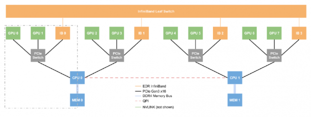
Figure 2: Networking topology of a DGX-1 server.
Figure 2 presents the layout of an NVIDIA DGX-1 server — we can think of this single box as a small supercomputer. The DGX-1 has eight P100 GPUs, four InfiniBand devices, and two CPUs. What is the most efficient route to take when passing data between GPU0 and GPU1? What about GPU2 and GPU7? GPU0 and GPU1 are connected via NVLink but GPU2 and GPU7 have direct communication lines, therefore, when passing data, we must perform two costly operations: Device-to-Host (moving data from GPU2 to the host) and Host-to-Device (moving data from the host to GPU7), and transferring data through main memory is expensive. Fortunately, a DGX-1 allows transfers between two GPUs that are not NVLink connected to use a more efficient transfer method than the costly operations described. With InfiniBand and GPUDirectRDMA, two GPUs can communicate without touching the main memory at all, allowing GPU7 to directly read GPU2’s memory via the InfiniBand interconnect only.
Referring back to Figure 1, you can now see why only using InfiniBand outperforms the NVLink connection alone — Host-to-Device/Device-to-Host transfers are costly! However, when combining InfiniBand with NVLink we achieve more optimal performance.
Further improvements
UCX-Py is under constant development, which means changes may occur without notice. Our ultimate commitment is to deliver high-performance communication to Python in a high-quality library package. With that said, we expect in the near future to keep on improving stability and ease-of-use, enabling users to benefit from enhanced performance with little to no effort to configure UCX-Py, thus automatically enabling accelerated communication hardware.
So far, we have tested UCX-Py mostly in DGX-1 and DGX-2 systems, where point-to-point and end-to-end performance was demonstrated. We scaled our testing up to one hundred Dask CUDA workers. We are constantly working to improve performance and stability, particularly for large scale workflows, and encourage users to engage with our team on GitHub and extend the discussion on UCX-Py.
What a gamer wants. What a gamer needs. Games that’ll make you happy and cloud gaming that’ll set you free … to play your favorite PC games anywhere, anytime, on GeForce NOW. Get a sneak peek of all the exciting games coming in June this GFN Thursday. Starting with titles launching today. Keeping It Fresh Read article >

 The 15 accepted papers and posters from NVIDIA range from simulating dynamic driving environments, to powering neural architecture search for medical imaging.


 The Clara AGX SDK runs on the NVIDIA Jetson and Clara AGX platform and provides developers with capabilities to build end-to-end streaming workflows for medical imaging.
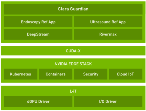
 NVIDIA Train, Adapt, and Optimize (TAO) is an AI model adaptation platform that simplifies and accelerates the creation of enterprise AI applications.
  Simulations are pervasive in every domain of science and engineering, but they are often constrained by large computational times, limited compute resources, tedious manual setup efforts, and the need for technical expertise. NVIDIA SimNet is a simulation toolkit that addresses these challenges with a combination of AI and physics. A success story of SimNet’s application …
 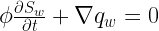 (1)
(1) is the porosity,
  is the saturation (or concentration) of that wetting phase, and is the saturation of the nonwetting. The flow rate of the wetting phase
  can be written as follows:
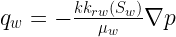 (2)
(2) is the absolute permeability that quantifies the propensity of a material to allow liquid or gas to flow through it.
  is the wetting phase relative permeability that is function of the saturation and characterizes the effective permeability of a given phase in the presence or absence of it. A phase preferentially flows through a path where it is already present. Think of a drop of water dripping down from a window and following existing trails.
 using a simple homogenization rule:
 ![q = -kleft[frac{k_{rw}(S_w)}{mu_w} + frac{k_{rn}(S_n)}{mu_n}right]nabla p](https://s0.wp.com/latex.php?latex=q+%3D+-k%5Cleft%5B%5Cfrac%7Bk_%7Brw%7D%28S_w%29%7D%7B%5Cmu_w%7D+%2B+%5Cfrac%7Bk_%7Brn%7D%28S_n%29%7D%7B%5Cmu_n%7D%5Cright%5D%5Cnabla+p&bg=ffffff&fg=000&s=2&c=20201002) (3)
(3) (4)
(4) (5)
(5) ), you can obtain the equation:
 (6)
(6) (7)
(7)  and
and  are the residual (irreducible) saturations for the wetting and nonwettings resulting from trapping mechanisms and
  is the endpoint mobility ratio defined as the ratio of endpoint-relative permeability and viscosity of both phases. We used the Corey and Brooks relative permeability relationship. For more information, see
 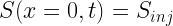 (8)
(8) (9)
(9)


 TL;DR UCX/UCX-Py is an accelerated networking library designed for low-latency high-bandwidth transfers for both host and GPU device memory objects. You can easily get started by installing through conda (limited to linux-64): Introduction RAPIDS is committed to delivering the highest achievable performance for the PyData ecosystem. There are now numerous GPU libraries for high-performance and …
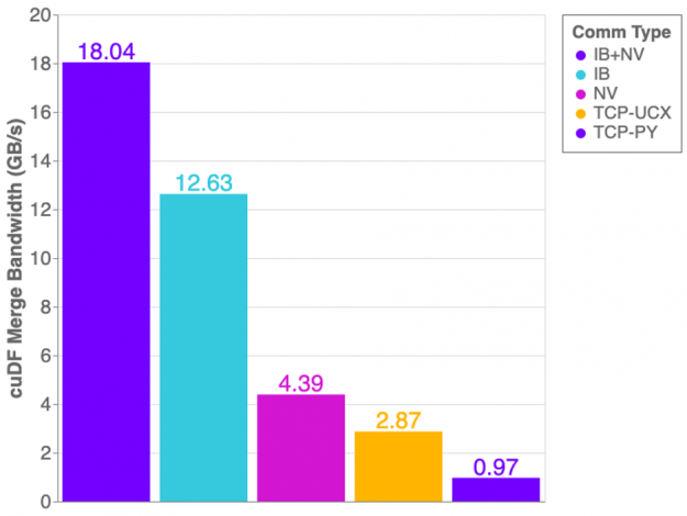