Posted by Jimmy (Tsung-Yen) Yang, Student Researcher, Robotics at Google
The promise of deep reinforcement learning (RL) in solving complex, high-dimensional problems autonomously has attracted much interest in areas such as robotics, game playing, and self-driving cars. However, effectively training an RL policy requires exploring a large set of robot states and actions, including many that are not safe for the robot. This is a considerable risk, for example, when training a legged robot. Because such robots are inherently unstable, there is a high likelihood of the robot falling during learning, which could cause damage.
The risk of damage can be mitigated to some extent by learning the control policy in computer simulation and then deploying it in the real world. However, this approach usually requires addressing the difficult sim-to-real gap, i.e., the policy trained in simulation can not be readily deployed in the real world for various reasons, such as sensor noise in deployment or the simulator not being realistic enough during training. Another approach to solve this issue is to directly learn or fine-tune a control policy in the real world. But again, the main challenge is to assure safety during learning.
In “Safe Reinforcement Learning for Legged Locomotion”, we introduce a safe RL framework for learning legged locomotion while satisfying safety constraints during training. Our goal is to learn locomotion skills autonomously in the real world without the robot falling during the entire learning process. Our learning framework adopts a two-policy safe RL framework: a “safe recovery policy” that recovers robots from near-unsafe states, and a “learner policy” that is optimized to perform the desired control task. The safe learning framework switches between the safe recovery policy and the learner policy to enable robots to safely acquire novel and agile motor skills.
The Proposed Framework
Our goal is to ensure that during the entire learning process, the robot never falls, regardless of the learner policy being used. Similar to how a child learns to ride a bike, our approach teaches an agent a policy while using “training wheels”, i.e., a safe recovery policy. We first define a set of states, which we call a “safety trigger set”, where the robot is close to violating safety constraints but can still be saved by a safe recovery policy. For example, the safety trigger set can be defined as a set of states with the height of the robots being below a certain threshold and the roll, pitch, yaw angles being too large, which is an indication of falls. When the learner policy results in the robot being within the safety trigger set (i.e., where it is likely to fall), we switch to the safe recovery policy, which drives the robot back to a safe state. We determine when to switch back to the learner policy by leveraging an approximate dynamics model of the robot to predict the future robot trajectory. For example, based on the position of the robot’s legs and the current angle of the robot based on sensors for roll, pitch, and yaw, is it likely to fall in the future? If the predicted future states are all safe, we hand the control back to the learner policy, otherwise, we keep using the safe recovery policy.
 |
| The state diagram of the proposed approach. (1) If the learner policy violates the safety constraint, we switch to the safe recovery policy. (2) If the learner policy cannot ensure safety in the near future after switching to the safe recovery policy, we keep using the safe recovery policy. This allows the robot to explore more while ensuring safety. |
This approach ensures safety in complex systems without resorting to opaque neural networks that may be sensitive to distribution shifts in application. In addition, the learner policy is able to explore states that are near safety violations, which is useful for learning a robust policy.
Because we use “approximated” dynamics to predict the future trajectory, we also examine how much safer a robot would be if we used a much more accurate model for its dynamics. We provide a theoretical analysis of this problem and show that our approach can achieve minimal safety performance loss compared to one with a full knowledge about the system dynamics.
Legged Locomotion Tasks
To demonstrate the effectiveness of the algorithm, we consider learning three different legged locomotion skills:
- Efficient Gait: The robot learns how to walk with low energy consumption and is rewarded for consuming less energy.
- Catwalk: The robot learns a catwalk gait pattern, in which the left and right two feet are close to each other. This is challenging because by narrowing the support polygon, the robot becomes less stable.
- Two-leg Balance: The robot learns a two-leg balance policy, in which the front-right and rear-left feet are in stance, and the other two are lifted. The robot can easily fall without delicate balance control because the contact polygon degenerates into a line segment.
 |
| Locomotion tasks considered in the paper. Top: efficient gait. Middle: catwalk. Bottom: two-leg balance. |
Implementation Details
We use a hierarchical policy framework that combines RL and a traditional control approach for the learner and safe recovery policies. This framework consists of a high-level RL policy, which produces gait parameters (e.g., stepping frequency) and feet placements, and pairs it with a low-level process controller called model predictive control (MPC) that takes in these parameters and computes the desired torque for each motor in the robot. Because we do not directly command the motors’ angles, this approach provides more stable operation, streamlines the policy training due to a smaller action space, and results in a more robust policy. The input of the RL policy network includes the previous gait parameters, the height of the robot, base orientation, linear, angular velocities, and feedback to indicate whether the robot is approaching the safety trigger set. We use the same setup for each task.
We train a safe recovery policy with a reward for reaching stability as soon as possible. Furthermore, we design the safety trigger set with inspiration from capturability theory. In particular, the initial safety trigger set is defined to ensure that the robot’s feet can not fall outside of the positions from which the robot can safely recover using the safe recovery policy. We then fine-tune this set on the real robot with a random policy to prevent the robot from falling.
Real-World Experiment Results
We report the real-world experimental results showing the reward learning curves and the percentage of safe recovery policy activations on the efficient gait, catwalk, and two-leg balance tasks. To ensure that the robot can learn to be safe, we add a penalty when triggering the safe recovery policy. Here, all the policies are trained from scratch, except for the two-leg balance task, which was pre-trained in simulation because it requires more training steps.
Overall, we see that on these tasks, the reward increases, and the percentage of uses of the safe recovery policy decreases over policy updates. For instance, the percentage of uses of the safe recovery policy decreases from 20% to near 0% in the efficient gait task. For the two-leg balance task, the percentage drops from near 82.5% to 67.5%, suggesting that the two-leg balance is substantially harder than the previous two tasks. Still, the policy does improve the reward. This observation implies that the learner can gradually learn the task while avoiding the need to trigger the safe recovery policy. In addition, this suggests that it is possible to design a safe trigger set and a safe recovery policy that does not impede the exploration of the policy as the performance increases.
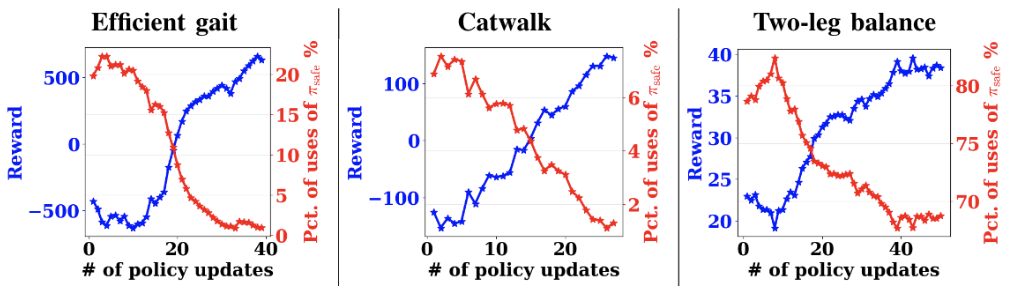 |
| The reward learning curve (blue) and the percentage of safe recovery policy activations (red) using our safe RL algorithm in the real world. |
In addition, the following video shows the learning process for the two-leg balance task, including the interplay between the learner policy and the safe recovery policy, and the reset to the initial position when an episode ends. We can see that the robot tries to catch itself when falling by putting down the lifted legs (front left and rear right) outward, creating a support polygon. After the learning episode ends, the robot walks back to the reset position automatically. This allows us to train policy autonomously and safely without human supervision.
 |
| Early training stage. |
 |
| Late training stage. |
 |
| Without a safe recovery policy. |
Finally, we show the clips of learned policies. First, in the catwalk task, the distance between two sides of the legs is 0.09m, which is 40.9% smaller than the nominal distance. Second, in the two-leg balance task, the robot can maintain balance by jumping up to four times via two legs, compared to one jump from the policy pre-trained from simulation.
 |
| Final learned two-leg balance. |
Conclusion
We presented a safe RL framework and demonstrated how it can be used to train a robotic policy with no falls and without the need for a manual reset during the entire learning process for the efficient gait and catwalk tasks. This approach even enables training of a two-leg balance task with only four falls. The safe recovery policy is triggered only when needed, allowing the robot to more fully explore the environment. Our results suggest that learning legged locomotion skills autonomously and safely is possible in the real world, which could unlock new opportunities including offline dataset collection for robot learning.
No model is without limitation. We currently ignore the model uncertainty from the environment and non-linear dynamics in our theoretical analysis. Including these would further improve the generality of our approach. In addition, some hyper-parameters of the switching criteria are currently being heuristically tuned. It would be more efficient to automatically determine when to switch based on the learning progress. Furthermore, it would be interesting to extend this safe RL framework to other robot applications, such as robot manipulation. Finally, designing an appropriate reward when incorporating the safe recovery policy can impact learning performance. We use a penalty-based approach that obtained reasonable results in these experiments, but we plan to investigate this in future work to make further performance improvements.
Acknowledgements
We would like to thank our paper co-authors: Tingnan Zhang, Linda Luu, Sehoon Ha, Jie Tan, and Wenhao Yu. We would also like to thank the team members of Robotics at Google for discussions and feedback.


 This Embedded Vision Summit session will showcase a low-code approach to develop fully optimized and accelerated vision AI applications using DeepStream SDK and graph composer.
  Learn to build and deploy a deep learning model for automated flood detection using satellite imagery in this new self-paced course from the NVIDIA Deep Learning Institute.


 The latest release of the NVIDIA DOCA software framework focuses on enhancements to DOCA infrastructure services.