I’m having a trained model of image classification which works fine on python but when i convert it to tflite and deploy on Android it gives different results Can anyone help me here
submitted by /u/shubham1300
[visit reddit] [comments]
 DataBloom
I’m having a trained model of image classification which works fine on python but when i convert it to tflite and deploy on Android it gives different results Can anyone help me here
submitted by /u/shubham1300
[visit reddit] [comments]

Hello I have been trying to create two tensorflow models to experiment with transfer learning. I have a trainned a cnn model for lung xray images for pneumonia(2 classes) by using the kaggle chest x-ray dataset .
Here is my code
import tensorflow as tf
import numpy as np
from tensorflow import keras
import os
from tensorflow.keras.preprocessing.image import ImageDataGenerator
from tensorflow.keras.preprocessing import image
import matplotlib.pyplot as plt
gen = ImageDataGenerator(rescale=1./255)
train_data = gen.flow_from_directory(“/Users/saibalaji/Downloads/chest_xray/train”,target_size=(500,500),batch_size=32,class_mode=’binary’)
test_data = gen.flow_from_directory(“/Users/saibalaji/Downloads/chest_xray/test”,target_size=(500,500),batch_size=32,class_mode=’binary’)
model = keras.Sequential()
# Convolutional layer and maxpool layer 1
model.add(keras.layers.Conv2D(32,(3,3),activation=’relu’,input_shape=(500,500,3)))
model.add(keras.layers.MaxPool2D(2,2))
# Convolutional layer and maxpool layer 2
model.add(keras.layers.Conv2D(64,(3,3),activation=’relu’))
model.add(keras.layers.MaxPool2D(2,2))
# Convolutional layer and maxpool layer 3
model.add(keras.layers.Conv2D(128,(3,3),activation=’relu’))
model.add(keras.layers.MaxPool2D(2,2))
# Convolutional layer and maxpool layer 4
model.add(keras.layers.Conv2D(128,(3,3),activation=’relu’))
model.add(keras.layers.MaxPool2D(2,2))
# This layer flattens the resulting image array to 1D array
model.add(keras.layers.Flatten())
# Hidden layer with 512 neurons and Rectified Linear Unit activation function
model.add(keras.layers.Dense(512,activation=’relu’))
# Output layer with single neuron which gives 0 for Cat or 1 for Dog
#Here we use sigmoid activation function which makes our model output to lie between 0 and 1
model.add(keras.layers.Dense(1,activation=’sigmoid’))
hist = model.compile(optimizer=’adam’,loss=’binary_crossentropy’,metrics=[‘accuracy’])
model.fit_generator(train_data,
steps_per_epoch = 163,
epochs = 4,
validation_data = test_data
)
I have saved the model in .h5 format.
Then I created a new notebook loaded data from kaggle for alzheimer’s disease and loaded my saved pneumonia model. Copied its layer to a new model except last layer then Freezed all the layers in the new model as non trainable. Then added a output dense layer with 4 neurons for 4 classes. Then trainned only the last layer for 5 epochs. But the problem is val accuaracy remains at 35% constant. How can I improve it.
Here is my code for alzeihmers model
import tensorflow as tf
from tensorflow import keras
from tensorflow.keras.preprocessing.image import ImageDataGenerator
from tensorflow.keras.preprocessing import image
import matplotlib.pyplot as plt
import numpy as np
gen = ImageDataGenerator(rescale=1./255)
traindata = datagen.flow_from_directory(‘/Users/saibalaji/Documents/TensorFlowProjects/ad/train’,target_size=(500,500),batch_size=32)
testdata = datagen.flow_from_directory(‘/Users/saibalaji/Documents/TensorFlowProjects/ad/test’,target_size=(500,500),batch_size=32)
model = keras.models.load_model(‘pn.h5’)
nmodel = keras.models.Sequential()
#add all layers except last one
for layer in model.layers[0:-1]:
nmodel.add(layer)
for layer in nmodel.layers:
layer.trainable = False
nmodel.add(keras.layers.Dense(units=4,name=’dense_last’))
hist = nmodel.compile(optimizer = tf.keras.optimizers.Adam(learning_rate=0.002),loss = ‘categorical_crossentropy’, metrics = [‘accuracy’])
nmodel.fit(x=traindata,validation_data=testdata,epochs=5,steps_per_epoch=160)
submitted by /u/kudoshinichi-8211
[visit reddit] [comments]
Automatic translation of speech from one language to speech in another language, called speech-to-speech translation (S2ST), is important for breaking down the communication barriers between people speaking different languages. Conventionally, automatic S2ST systems are built with a cascade of automatic speech recognition (ASR), text-to-text machine translation (MT), and text-to-speech (TTS) synthesis sub-systems, so that the system overall is text-centric. Recently, work on S2ST that doesn’t rely on intermediate text representation is emerging, such as end-to-end direct S2ST (e.g., Translatotron) and cascade S2ST based on learned discrete representations of speech (e.g., Tjandra et al.). While early versions of such direct S2ST systems obtained lower translation quality compared to cascade S2ST models, they are gaining traction as they have the potential both to reduce translation latency and compounding errors, and to better preserve paralinguistic and non-linguistic information from the original speech, such as voice, emotion, tone, etc. However, such models usually have to be trained on datasets with paired S2ST data, but the public availability of such corpora is extremely limited.
To foster research on such a new generation of S2ST, we introduce a Common Voice-based Speech-to-Speech translation corpus, or CVSS, which includes sentence-level speech-to-speech translation pairs from 21 languages into English. Unlike existing public corpora, CVSS can be directly used for training such direct S2ST models without any extra processing. In “CVSS Corpus and Massively Multilingual Speech-to-Speech Translation”, we describe the dataset design and development, and demonstrate the effectiveness of the corpus through training of baseline direct and cascade S2ST models and showing performance of a direct S2ST model that approaches that of a cascade S2ST model.
Building CVSS
CVSS is directly derived from the CoVoST 2 speech-to-text (ST) translation corpus, which is further derived from the Common Voice speech corpus. Common Voice is a massively multilingual transcribed speech corpus designed for ASR in which the speech is collected by contributors reading text content from Wikipedia and other text corpora. CoVoST 2 further provides professional text translation for the original transcript from 21 languages into English and from English into 15 languages. CVSS builds on these efforts by providing sentence-level parallel speech-to-speech translation pairs from 21 languages into English (shown in the table below).
To facilitate research with different focuses, two versions of translation speech in English are provided in CVSS, both are synthesized using state-of-the-art TTS systems, with each version providing unique value that doesn’t exist in other public S2ST corpora:
Together with the source speech, the two S2ST datasets contain 1,872 and 1,937 hours of speech, respectively.
| Source Language |
Code | Source speech (X) |
CVSS-C target speech (En) |
CVSS-T target speech (En) |
| French | fr | 309.3 | 200.3 | 222.3 |
| German | de | 226.5 | 137.0 | 151.2 |
| Catalan | ca | 174.8 | 112.1 | 120.9 |
| Spanish | es | 157.6 | 94.3 | 100.2 |
| Italian | it | 73.9 | 46.5 | 49.2 |
| Persian | fa | 58.8 | 29.9 | 34.5 |
| Russian | ru | 38.7 | 26.9 | 27.4 |
| Chinese | zh | 26.5 | 20.5 | 22.1 |
| Portuguese | pt | 20.0 | 10.4 | 11.8 |
| Dutch | nl | 11.2 | 7.3 | 7.7 |
| Estonian | et | 9.0 | 7.3 | 7.1 |
| Mongolian | mn | 8.4 | 5.1 | 5.7 |
| Turkish | tr | 7.9 | 5.4 | 5.7 |
| Arabic | ar | 5.8 | 2.7 | 3.1 |
| Latvian | lv | 4.9 | 2.6 | 3.1 |
| Swedish | sv | 4.3 | 2.3 | 2.8 |
| Welsh | cy | 3.6 | 1.9 | 2.0 |
| Tamil | ta | 3.1 | 1.7 | 2.0 |
| Indonesian | id | 3.0 | 1.6 | 1.7 |
| Japanese | ja | 3.0 | 1.7 | 1.8 |
| Slovenian | sl | 2.9 | 1.6 | 1.9 |
| Total | 1,153.2 | 719.1 | 784.2 | |
| Amount of source and target speech of each X-En pair in CVSS (hours). |
In addition to translation speech, CVSS also provides normalized translation text matching the pronunciation in the translation speech (on numbers, currencies, acronyms, etc., see data samples below, e.g., where “100%” is normalized as “one hundred percent” or “King George II” is normalized as “king george the second”), which can benefit both model training as well as standardizing the evaluation.
CVSS is released under the Creative Commons Attribution 4.0 International (CC BY 4.0) license and it can be freely downloaded online.
Data Samples
| Example 1: | ||
| Source audio (French) | ||
| Source transcript (French) | Le genre musical de la chanson est entièrement le disco. | |
| CVSS-C translation audio (English) | ||
| CVSS-T translation audio (English) | ||
| Translation text (English) | The musical genre of the song is 100% Disco. | |
| Normalized translation text (English) | the musical genre of the song is one hundred percent disco | |
| Example 2: | ||
| Source audio (Chinese) | ||
| Source transcript (Chinese) | 弗雷德里克王子,英国王室成员,为乔治二世之孙,乔治三世之幼弟。 | |
| CVSS-C translation audio (English) | ||
| CVSS-T translation audio (English) | ||
| Translation text (English) | Prince Frederick, member of British Royal Family, Grandson of King George II, brother of King George III. | |
| Normalized translation text (English) | prince frederick member of british royal family grandson of king george the second brother of king george the third | |
Baseline Models
On each version of CVSS, we trained a baseline cascade S2ST model as well as two baseline direct S2ST models and compared their performance. These baselines can be used for comparison in future research.
Cascade S2ST: To build strong cascade S2ST baselines, we trained an ST model on CoVoST 2, which outperforms the previous states of the art by +5.8 average BLEU on all 21 language pairs (detailed in the paper) when trained on the corpus without using extra data. This ST model is connected to the same TTS models used for constructing CVSS to compose very strong cascade S2ST baselines (ST → TTS).
Direct S2ST: We built two baseline direct S2ST models using Translatotron and Translatotron 2. When trained from scratch with CVSS, the translation quality from Translatotron 2 (8.7 BLEU) approaches that of the strong cascade S2ST baseline (10.6 BLEU). Moreover, when both use pre-training the gap decreases to only 0.7 BLEU on ASR transcribed translation. These results verify the effectiveness of using CVSS to train direct S2ST models.
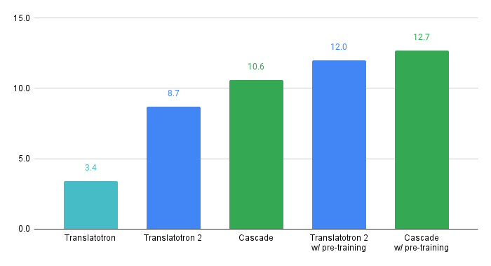 |
| Translation quality of baseline direct and cascade S2ST models built on CVSS-C, measured by BLEU on ASR transcription from speech translation. The pre-training was done on CoVoST 2 without other extra data sets. |
Conclusion
We have released two versions of multilingual-to-English S2ST datasets, CVSS-C and CVSS-T, each with about 1.9K hours of sentence-level parallel S2ST pairs, covering 21 source languages. The translation speech in CVSS-C is in a single canonical speaker’s voice, while the same in CVSS-T is in voices transferred from the source speech. Each of these datasets provides unique value not existing in other public S2ST corpora.
We built baseline multilingual direct S2ST models and cascade S2ST models on both datasets, which can be used for comparison in future works. To build strong cascade S2ST baselines, we trained an ST model on CoVoST 2, which outperforms the previous states of the art by +5.8 average BLEU when trained on the corpus without extra data. Nevertheless, the performance of the direct S2ST models approaches the strong cascade baselines when trained from scratch, and with only 0.7 BLEU difference on ASR transcribed translation when utilized pre-training. We hope this work helps accelerate the research on direct S2ST.
Acknowledgments
We acknowledge the volunteer contributors and the organizers of the Common Voice and LibriVox projects for their contribution and collection of recordings, the creators of Common Voice, CoVoST, CoVoST 2, Librispeech and LibriTTS corpora for their previous work. The direct contributors to the CVSS corpus and the paper include Ye Jia, Michelle Tadmor Ramanovich, Quan Wang, Heiga Zen. We also thank Ankur Bapna, Yiling Huang, Jason Pelecanos, Colin Cherry, Alexis Conneau, Yonghui Wu, Hadar Shemtov and Françoise Beaufays for helpful discussions and support.

 The article includes a step by step explanation of the merge sort algorithm and code snippets illustrating the implementation of the algorithm itself.
Data Scientists deal with algorithms daily. However, the data science discipline as a whole has developed into a role that does not involve implementation of sophisticated algorithms. Nonetheless, practitioners can still benefit from building an understanding and repertoire of algorithms.
In this article, the sorting algorithm merge sort is introduced, explained, evaluated, and implemented. The aim of this post is to provide you with robust background information on the merge sort algorithm, which acts as foundational knowledge for more complicated algorithms.
Although merge sort is not considered to be complex, understanding this algorithm will help you recognize what factors to consider when choosing the most efficient algorithm to perform data-related tasks. Created in 1945, John Von Neumann developed the merge sort algorithm using the divide-and-conquer approach.
To understand the merge sort algorithm, you must be familiar with the divide and conquer paradigm, alongside the programming concept of recursion. Recursion within the computer science domain is when a method defined to solve a problem involves an invocation of itself within its implementation body.
In other words, the function calls itself repeatedly.

Divide and conquer algorithms (which merge sort is a type of) employ recursion within its approach to solve specific problems. Divide and conquer algorithms decompose complex problems into smaller sub-parts, where a defined solution is applied recursively to each sub-part. Each sub-part is then solved separately, and the solutions are recombined to solve the original problem.
The divide-and-conquer approach to algorithm design combines three primary elements:
Other algorithms use the divide-and-conquer paradigm, such as Quicksort, Binary Search, and Strassen’s algorithm.
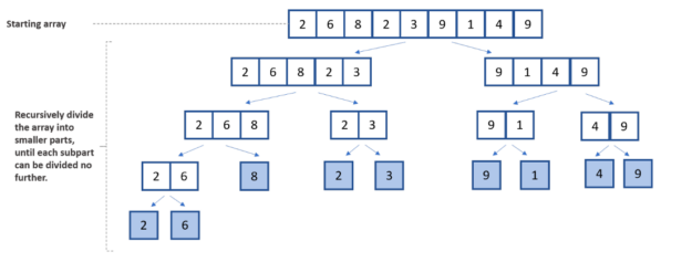
In the context of sorting elements in a list and in ascending order, the merge sort method divides the list into halves, then iterates through the new halves, continually dividing them down further to their smaller parts.
Subsequently, a comparison of smaller halves is conducted, and the results are combined together to form the final sorted list.
Implementation of the merge sort algorithm is a three-step procedure. Divide, conquer, and combine.
The divide component of the divide-and-conquer approach is the first step. This initial step separates the overall list into two smaller halves. Then, the lists are broken down further until they can no longer be divided, leaving only one element item in each halved list.
The recursive loop in merge sort’s second phase is concerned with the list’s elements being sorted in a particular order. For this scenario, the initial array is sorted in ascending order.
In the following illustration, you can see the division, comparison, and combination steps involved in the merge sort algorithm.

To implement this yourself:
def merge_sort(list: [int]):
    list_length = len(list)

    if list_length == 1:
        return list

    mid_point = list_length // 2

    left_half = merge_sort(list[:mid_point])
    right_half = merge_sort(list[mid_point:])

return merge(left_half, right_half)def merge(left, right):
output = []
i = j = 0
while (i Big O notation is a standard for defining and organizing the performance of algorithms in terms of their space requirement and execution time.
Merge sort algorithm time complexity is the same for its best, worst, and average scenarios. For a list of size n, the expected number of steps, minimum number of steps, and maximum number of steps for the merge sort algorithm to complete, are all the same.
As noted earlier in this article, the merge sort algorithm is a three-step process: divide, conquer, and combine. The ‘divide’ step involves the computation of the midpoint of the list, which, regardless of the list size, takes a single operational step. Therefore the notation for this operation is denoted as O(1).
The ‘conquer’ step involves dividing and recursively solving subarrays–the notation log n denotes this. The ‘combine’ step consists of combining the results into a final list; this operation execution time is dependent on the list size and denoted as O(n).
The merge sort notation for its average, best, and worst time complexity is log n * n * O(1). In Big O notation, low-order terms and constants are negligible, meaning the final notation for the merge sort algorithm is O(n log n). For a detailed analysis of the merge sort algorithm, refer to this article.
Merge sort performs well when sorting large lists, but its operation time is slower than other sorting solutions when used on smaller lists. Another disadvantage of merge sort is that it will execute the operational steps even if the initial list is already sorted. In the use case of sorting linked lists, merge sort is one of the fastest sorting algorithms to use. Merge sort can be used in file sorting within external storage systems, such as hard drives.
This article describes the merge sort technique by breaking it down in terms of its constituent operations and step-by-step processes.
Merge sort algorithm is commonly used and the intuition and implementation behind the algorithm is rather straightforward in comparison to other sorting algorithms. This article includes the implementation step of the merge sort algorithm in Python.
You should also know that the time complexity of the merge sort method’s execution time in different situations, remains the same for best, worst, and average scenarios. It is recommended that merge sort algorithm is applied in the following scenarios:
Hello everyone,
I’m pretty new to ML and tensorflow. What I’m trying to do now is practically to inverse a function using tensorflow.
So I have a function h=f(c1, c2,..cn, T). It is a smooth function of all the variables. I want to train a model which would give me T given known values of c1…cn and h.
For now I’m using a keras.Sequential model with 2 or 3 dense layers.
For loss I use ‘mean_absolute_error’, For optimizer – Adam().
To train the model I generate a dataset using my h(c1…cn, T) function by varying its arguments and using values of T as train_labels.
The accuracy of the resulting model is not very good to my mind – I’m getting errors of about 10%. To my mind this is not very good, given that the training dataset is ideally smooth.
My questions are:
Am I doing something particularly wrong?
How many units should I provide for each layer? I mean in tutorials they are using either Dense(64) or Dense(1). What difference does it make in my particular case? Should it be proportional to the number of parameters of the model?
May be I should use some other types of layers/optimizers/losses?
Thank you in advance for your replies!
submitted by /u/_padla_
[visit reddit] [comments]
I’m planning to build a model that uses ParameterServerStrategy to distribute its parameters across multiple VMs with an assumption that it cannot fit into any one of the VMs. Is it possible to use TensorFlow serving to distribute the model across multiple VMs?
I was reading through this (https://www.tensorflow.org/tfx/serving/architecture) and I discovered that you need multiple servables for composite models that have multiple parts to them. But I couldn’t find any documentation that talks specifically about creating a cluster with tf serving, that uses multiple servables with each servable in a single VM.
Is it possible to use TensorFlow serving for very large models, where the models have its parameters spread across multiple VMs? If yes, can you please tell me how it can be done?
Thanks in advance!
submitted by /u/deathconqueror
[visit reddit] [comments]
In addition to GFN Thursday, it’s National Tater Day. Hooray! To honor the spud-tacular holiday, we’re closing out March with seven new games streaming this week. And a loaded 20+ titles are coming to the GeForce NOW library in April to play — even on a potato PC, thanks to GeForce NOW. Plus, the GeForce Read article >
The post An A-peel-ing GFN Thursday Sprouts 20+ New Games Coming to GeForce NOW in April appeared first on NVIDIA Blog.
Hi, very fresh to ML in general, I’m overwhelmed by choice for loss functions and accuracy measurements. Doing my masters project and my supervisor wants me to teach myself tf and throw the data through a model.
I’m feeding in an array of particle data from a decay, and asking for it to predict a 1 or -1 at the end representing parity of the original particle.
What loss fn and accuracy metric is best to use for something like this.
Other parameters, about 2 million events, 6particles in each decay/event. Their 4 momenta in each. That makes 24 in put strings.
First layer is a tf.flatten,
submitted by /u/DriftingRumour
[visit reddit] [comments]
I am trying to have a layer with only positive weights generate a partially negative output. What would the least hacky way to achieve this be? My initial idea was using a modified activation function that is shifted by 1 along the x axis, however, this feels a bit hacky to me and I was wondering if there was a better way to achieve this
submitted by /u/salted_kinase
[visit reddit] [comments]
Hi Guys,
Is there a way to store a tensor in multiple GPUs? I have a tensor that is so large that requires >16Gb of GPU RAM to store. I was wonder how that can be achieved. Thanks!
submitted by /u/dr_meme_69
[visit reddit] [comments]