
 Great sessions on custom computer vision models, expressive TTS, localized NLP, scalable recommenders, and commercial and healthcare robotics apps.
Looking for different topic areas? Keep an eye out for our other posts!
Join us at GTC, March 21-24, to explore the latest technology and research across AI, computer vision, data science, robotics, and more!
With over 900 options to choose from, our NVIDIA experts put together some can’t-miss sessions to help get you started:
Computer Vision / Video Analytics
Creating the Future: Creating the World’s Largest Synthetic Object Recognition Dataset for Industry (SORDI)
Jimmy Nassif, CTO, idealworks
Marc Kamradt, Head of TechOffice MUNICH, BMW Group
BMW builds a car every 56 seconds. How do they increase quality? They use robots and complement real data with synthetic. Learn how BMW, Microsoft, and NVIDIA are accelerating production and quality by recognizing parts, obstacles, and people through artificial intelligence-based computer vision.
How To Develop and Optimize Edge AI apps with NVIDIA DeepStream
Carlos Garcia-Sierra, DeepStream Product Manager, NVIDIA
Jitendra Kumar, Senior System Software Engineer, NVIDIA
This talk covers the best practices for developing and optimizing the performance of edge AI applications using DeepStream SDK. Deep dive into a multisensor, multimodel design and learn how to reduce development time and maximize performance using AI at the edge.
AI Models Made Simple with NVIDIA TAO
Chintan Shah, Senior Product Manager, NVIDIA
Akhil Docca, Senior Product Marketing Manager, NVIDIA
A primary challenge confronting enterprises is the demand for creating AI models far outpaces the number of data scientists available. Developers need to easily customize models and bring their AI to market faster. This session will demonstrate the power and ease of NVIDIA TAO that solves this problem. Get a preview at GTC for the new capabilities of TAO Toolkit, including Bring Your Own Model Weights, Rest APIs, TensorBoard visualization, new pretrained models, and more.
Conversational AI / NLP
Conversational AI Demystified
Sirisha Rella, Product Marketing Manager, NVIDIA
It’s easier than ever to develop AI speech applications like virtual assistants and real-time transcription. Today’s advanced tools and technologies make it easy to fine-tune and build scalable, responsive applications. This popular session shows users how to build and deploy their first end-to-end conversational AI pipeline using NVIDIA Riva, as an example.
Expressive Neural Text-to-Speech
Andrew Breen, Senior Manager Text-to-Speech Research, Amazon
Text-to-speech (TTS) research expert Andrew Breen will give a high-level overview of recent developments in neural TTS, including adopted approaches, technical challenges, and future direction. Breen was awarded the IEE J. Langham Thomson premium in 1993, and has received business awards from BT, MCI, and Nuance. He invented the Laureate TTS system at BT Labs and founded Nuance’s TTS organization.
Building Large-scale, Localized Language Models: From Data Preparation to Training and Deployment to Production
Miguel Martinez, Senior Deep Learning Solution Architect, NVIDIA
Meriem Bendris, Senior Deep Learning Data Scientist, NVIDIA
Natural Language Processing (NLP) breakthroughs in large-scale language models have boosted the capability to solve problems with zero-shot translation and supervised fine-tuning. However, executing NLP models on localized languages remains limited due to data preparation, training, and deployment challenges. This session highlights scaling challenges and solutions to show how to optimize NLP models using NVIDIA NeMo Megatron—a framework for training large NLP models in other languages.
Recommenders / Personalization
Building and Deploying Recommender Systems Quickly and Easily with NVIDIA Merlin
Even Oldridge, Senior Manager, Merlin Recommender Systems Team, NVIDIA
Merlin expert and Twitter influencer Even Oldridge will demonstrate how to optimize recommendation models for maximum performance and scale. Olrdige is a Twitter influencer and has 8 years of recommender system experience, along with a PhD in computer vision.
Building AI-based Recommender System Leveraging the Power of Deep Learning and GPU
Khalifeh AlJadda, Senior Director of Data Science, The Home Depot
Tackle AI-based recommendation system challenges and uncover best practices for delivering personalized experiences that differentiate you from competitors. Hear from Khalifeh AlJadda, an expert in implementing large-scale, distributed, machine-learning algorithms in search and recommendation engines. AlJadda leads the Recommendation Data Science, Search Data Science, and Visual AI teams at The Home Depot. With a PhD in computer science, he previously led the design and implementation of CareerBuilder’s language-agnostic semantic search engine.
Multi-Objective Optimization to Boost Exploration in Recommender Systems
Serdar Kadioglu, Vice President AI | Adjunct Assistant Professor, Fidelity Investments | Brown University
How can one use combinatorial optimization to formalize item universe selection in new applications with limited or no datasets? Serdar Kadioglu, will provide insights on how to apply techniques like unsupervised clustering and latent text embeddings to create a multilevel framework for your business. Kadioglu previously led the Advanced Constraint Technology R&D team at Oracle and worked at Adobe. As an adjunct professor at Brown University for computer science, Kadioglu’s algorithmic research is at the intersection of AI and discrete optimization with an interest in building robust and scalable products.
Robotics
Delivering AI Robotics at Scale: A Behind-the-Scenes Look
Mostafa Rohaninejad, Founding Researcher, Covariant.ai
Bringing practical AI robotics into the physical world, such as on a factory floor, is hard. Covariant is working to solve this problem. Mostafa Rohaninejad is part of the core team that built the full AI stack at Covariant from the ground up. In his session, he will share both the technical challenges and the exciting commercial possibilities of AI Robotics.
Leveraging Embedded Computing to Unlock Autonomy in Human Environments
Andrea Thomaz, Co-Founder and CEO, Diligent Robotics
During the COVID-19 pandemic, hospitals faced high nurse turnover, record burnout, and crisis-level labor shortages. Hospitals must alleviate this staffing crisis. Enter Diligent Robotics, and their robot Moxi, which completes routine tasks to assist nursing staff. Andrea Thomaz will share the unique challenges in achieving robot autonomy in a busy hospital, like maneuvering around objects or navigating to a patient room, all while integrating multiple camera streams that feed into embedded GPUs.
Building Autonomy Off-Road from the Ground Up with Jetson
Nick Peretti, CV/ML Engineer, Scythe Robotics
Autonomy is critical when it comes to outdoor and off-road robotics, but environmental and task-specific demands require a different approach than indoor or on-road environments. Nick Peretti will share the NVIDIA Jetson-centered approach that Scythe Robotics uses to run its full sense-plan-act software suite with their autonomous commercial mowers. He will highlight tools and approaches that have enabled Scythe to move quickly to field units, and lessons learned along the way.


 Is your network getting long in the tooth and are you thinking about an upgrade? This blog will cover three areas to consider when updating your data center network.


 AWS and NVIDIA collaborated on Bottlerocket, a container-optimized OS, to support all NVIDIA powered Amazon EC2 instances like the P4d, P3, G4dn, and G5 instances.
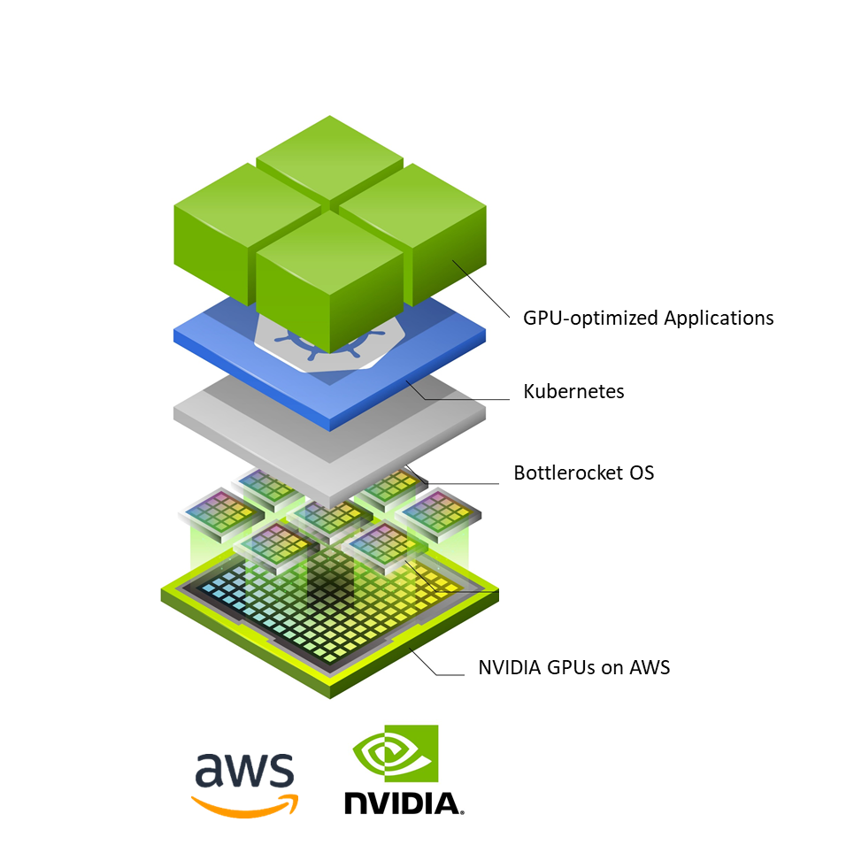