Posted by Ali Kemal Sinop and Kostas Kollias, Research Scientists, Google Research
In the world of networks, there are models that can explain observations across a diverse collection of applications. These include simple tasks such as computing the shortest path, which has obvious applications to routing networks but also applies in biology, e.g., where the slime mold Physarum is able to find shortest paths in mazes. Another example is Braess’s paradox — the observation that adding resources to a network can have an effect opposite to the one expected — which manifests not only in road networks but also in mechanical and electrical systems. For instance, constructing a new road can increase traffic congestion or adding a new link in an electrical circuit can increase voltage. Such connections between electrical circuits and other types of networks have been exploited for various tasks, such as partitioning networks, and routing flows.
In “Robust Routing Using Electrical Flows”, which won the Best Paper Award at SIGSPATIAL 2021, we present another interesting application of electrical flows in the context of road network routing. Specifically, we utilize ideas from electrical flows for the problem of constructing multiple alternate routes between a given source and destination. Alternate routes are important for many use cases, including finding routes that best match user preferences and for robust routing, e.g., routing that guarantees finding a good path in the presence of traffic jams. Along the way, we also describe how to quickly model electrical flows on road networks.
Existing Approaches to Alternate Routing
Computing alternate routes on road networks is a relatively new area of research and most techniques rely on one of two main templates: the penalty method and the plateau method. In the former, alternate routes are iteratively computed by running a shortest path algorithm and then, in subsequent runs, adding a penalty to those segments already included in the shortest paths that have been computed, to encourage further exploration. In the latter, two shortest path trees are built simultaneously, one starting from the origin and one from the destination, which are used to identify sequences of road segments that are common to both trees. Each such common sequence (which are expected to be important arterial streets for example) is then treated as a visit point on the way from the origin to the destination, thus potentially producing an alternate route. The penalty method is known to produce results of high quality (i.e., average travel time, diversity and robustness of the returned set of alternate routes) but is very slow in practice, whereas the plateau method is much faster but results in lower quality solutions.
An Alternate to Alternate Routing: Electrical Flows
Our approach is different and assumes that a routing problem on a road network is in many ways analogous to the flow of electrical current through a resistor network. Though the electrical current travels through many different paths, it is weaker along paths of higher resistance and stronger on low resistance ones, all else being equal.
We view the road network as a graph, where intersections are nodes and roads are edges. Our method then models the graph as an electrical circuit by replacing the edges with resistors, whose resistances equal the road traversal time, and then connecting a battery to the origin and destination, which results in electrical current between those two points. In this analogy, the resistance models how time-consuming it is to traverse a segment. In this sense, long and congested segments have high resistances. Intuitively speaking, the flow of electrical current will be spread around the entire network but concentrated on the routes that have lower resistance, which correspond to faster routes. By identifying the primary routes taken by the current, we can construct a viable set of alternates from origin to destination.
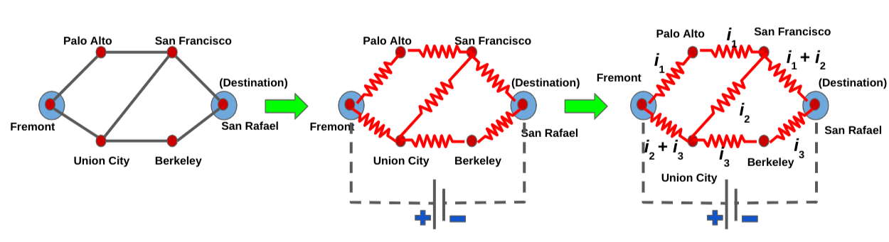 |
| Example of how we construct the electrical circuit corresponding to the road network. The current can be decomposed into three flows, i1, i2 and i3; each of which corresponds to a viable alternate path from Fremont to San Rafael. |
In order to compute the electrical flow, we use Kirchhoff’s and Ohm’s laws, which say respectively: 1) the algebraic sum of currents at each junction is equal to zero, meaning that the traffic that enters any intersection also exits it (for instance if three cars enter an intersection from one street and another car enters the same intersection from another street, a total of four cars need to exit the intersection); and 2) the current is directly proportional to the voltage difference between endpoints. If we write down the resulting equations, we end up with a linear system with n equations over n variables, which correspond to the potentials (i.e, the voltage) at each intersection. While voltage has no direct analogy to road networks, it can be used to help compute the flow of electrical current and thus find alternate routes as described above.
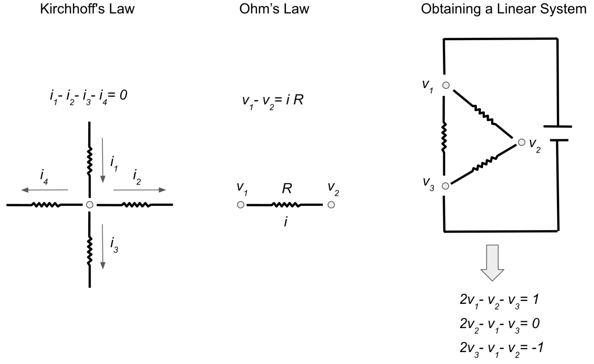 |
| In order to find the electrical current i (or flow) on each wire, we can use Kirchhoff’s law and Ohm’s law to obtain a linear system of equations in terms of voltages (or potentials) v. This yields a linear system with three equations (representing Kirchhoff’s law) and three unknowns (voltages at each intersection). |
So the computation boils down to computing values for the variables of this linear system involving a very special matrix called Laplacian matrix. Such matrices have many useful properties, e.g., they are symmetric and sparse — the number of off-diagonal non-zero entries is equal to twice the number of edges. Even though there are many existing near-linear time solvers for such systems of linear equations, they are still too slow for the purposes of quickly responding to routing requests with low latency. Thus we devised a new algorithm that solves these linear systems much faster for the special case of road networks1.
Fast Electrical Flow Computation
The first key part of this new algorithm involves Gaussian elimination, which is possibly the most well-known method for solving linear systems. When performed on a Laplacian matrix corresponding to some resistor network, it corresponds to the Y-Δ transformation, which reduces the number of nodes, while preserving the voltages. The only downside is that the number of edges may increase, which would make the linear system even slower to solve. For example, if a node with 10 connections is eliminated using the Y-Δ transformation, the system would end up with 35 new connections!
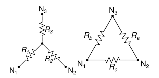 |
| The Y-Δ transformation allows us to remove the middle junction and replace it with three connections (Ra, Rb and Rc) between N1, N2 and N3. (Image from Wikipedia) |
However if one can identify parts of the network that are connected to the rest through very few nodes (lets call these connections bottlenecks), and perform elimination on everything else while leaving the bottleneck nodes, the new edges formed at the end will only be between bottleneck nodes. Provided that the number of bottleneck nodes is much smaller than the number of nodes eliminated with Y-Δ — which is true in the case of road networks since bottleneck nodes, such as bridges and tunnels, are much less common than regular intersections — this will result in a large net decrease (e.g., ~100x) in terms of graph size. Fortunately, identifying such bottlenecks in road networks can be done easily by partitioning such a network. By applying Y-Δ transformation to all nodes except the bottlenecks2, the result is a much smaller graph for which the voltages can be solved faster.
But what about computing the currents on the rest of the network, which is not made up of bottleneck nodes? A useful property about electrical flows is that once the voltages on bottleneck nodes are known, one can easily compute the electrical flow for the rest of the network. The electrical flow inside a part of the network only depends on the voltage of bottleneck nodes that separate that part from the rest of the network. In fact, it’s possible to precompute a small matrix so that one can recover the electrical flow by a single matrix-vector multiplication, which is a very fast operation that can be run in parallel.
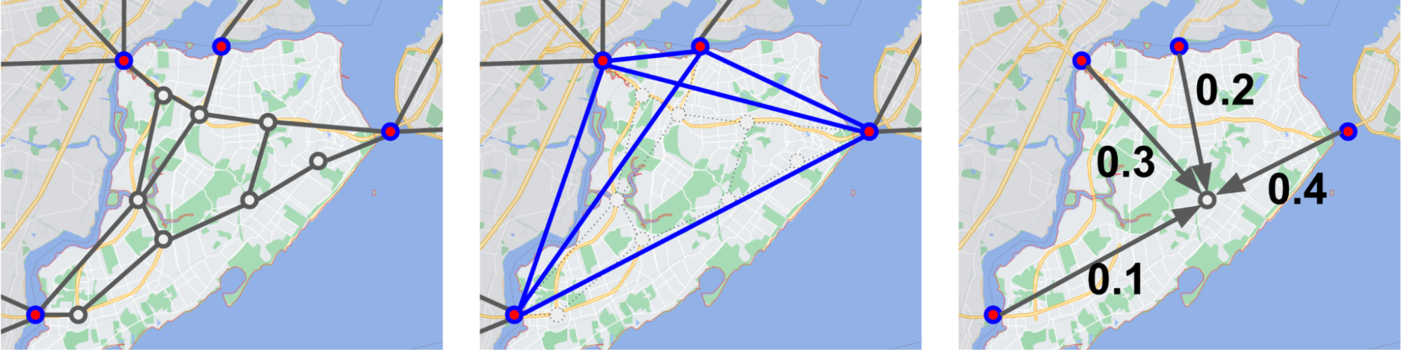 |
| Consider the imposed conceptual road network on Staten Island (left), for which directly computing the electrical flow would be slow. The bridges (red nodes) are the bottleneck points, and we can eliminate the whole road network inside the island by repeatedly applying Gaussian Elimination (or Y-Δ transformation). The resulting network (middle) is a much smaller graph, which allows for faster computation. The potentials inside the eliminated part are always a fixed linear combination of the bottleneck nodes (right). |
Once we obtain a solution that gives the electrical flow in our model network, we can observe the routes that carry the highest amount of electrical flow and output those as alternate routes for the road network.
Results
Here are some results depicting the alternates computed by the above algorithm.
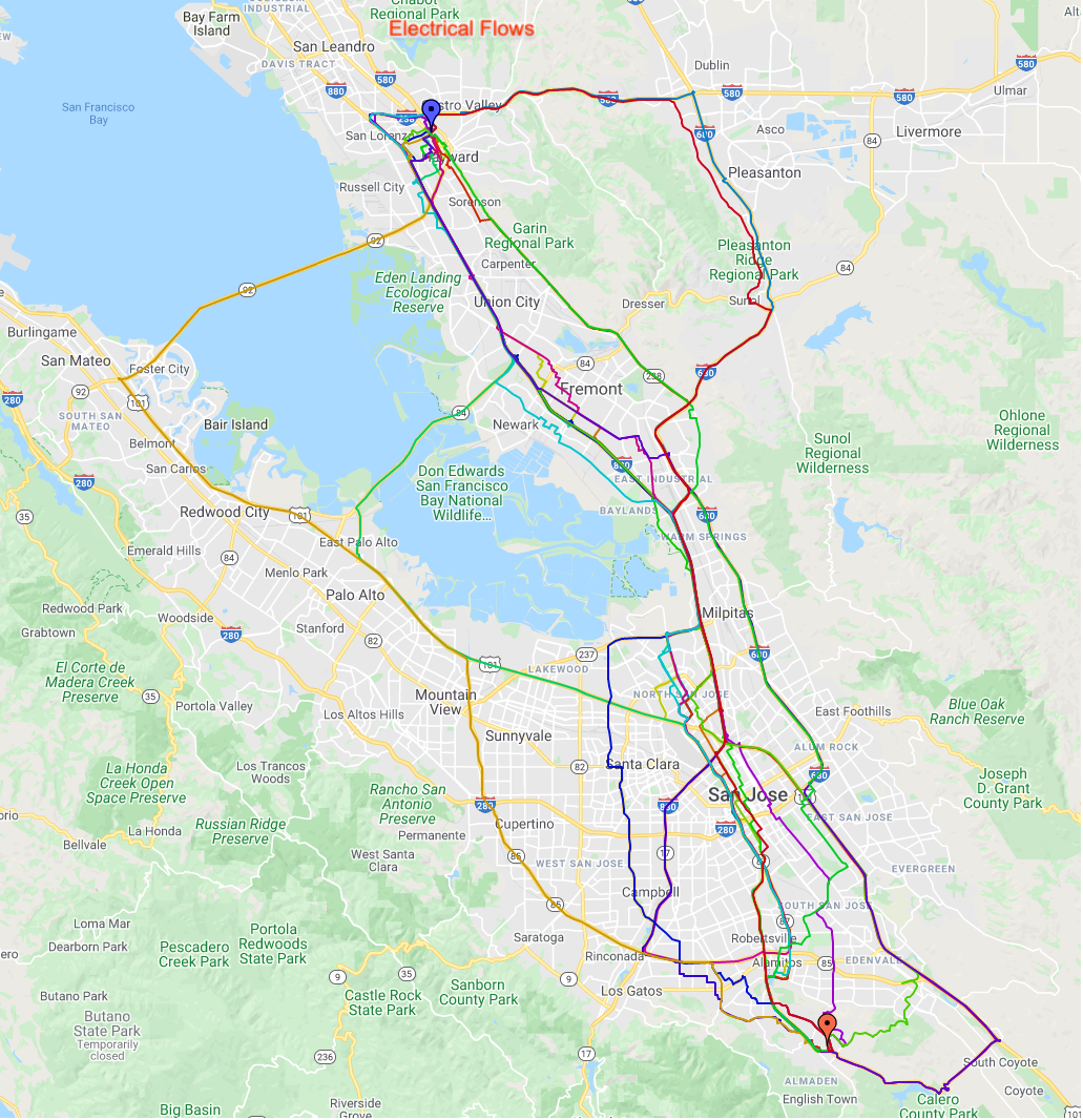 |
| Different alternates found for the Bay Area. Different colors correspond to different routes from the origin (red icon toward the bottom) to the destination (blue icon toward the top). |
Conclusion
In this post we describe a novel approach for computing alternate routes in road networks. Our approach is fundamentally different from the main techniques applied in decades of research in the area and provides high quality alternate routes in road networks by studying the problem through the lens of electrical circuits. This is an approach that can prove very useful in practical systems and we hope inspires more research in the area of alternate route computation and related problems. Interested readers can find a more detailed discussion of this work in our SIGSPATIAL 2021 talk recording.
Acknowledgements
We thank our collaborators Lisa Fawcett, Sreenivas Gollapudi, Ravi Kumar, Andrew Tomkins and Ameya Velingker from Google Research.
1Our techniques work for any network that can be broken down to smaller components with the removal of a few nodes. ↩
2 Performing Y-Δ transformation one-by-one for each node will be too slow. Instead we eliminate whole groups of nodes by taking advantage of the algebraic properties of Y-Δ transformation. ↩