This post details the latest functionality of RAPIDS Accelerator for Apache Spark.
RAPIDS Accelerator for Apache Spark v21.10 is now available! As an open source project, we value our community, their voice, and requests. This release constitutes community requests for operations that are ideally suited for GPU acceleration.
Important callouts for this release:
Speed up – performance improvements and cost savings.
New Functionality – new I/O and nested datatype Qualification and Profiling tool features.
RAPIDS Accelerator for Apache Spark is growing at a great pace in both functionality and performance. Standard industry benchmarks are a great way to measure performance over a period of time but another barometer to measure performance is to measure performance of common operators that are used in the data preprocessing stage or in data analytics.
We used four such queries shown in the chart below:
Count Distinct: a function used to estimate the number of unique page views or unique customers visiting an e-commerce site.
Window: a critical operator necessary for preprocessing components in analyzing timestamped event data in marketing or financial industry.
Intersect: an operator used to remove duplicates in a dataframes.
Cross-join: A common use for a cross join is to obtain all combinations of items.
These queries were run on a Google Cloud Platform (GCP) machine with 2xT4 GPUs each with 104GB RAM. The dataset used was of size 3TB with multiple different data types. More information about the setup and the queries can be found in the spark-rapids-examples repository on GitHub. These four queries show not only performance and cost benefits but also the range of speed-up (27x to 1.5x) varies depending on compute intensity. These queries vary in compute and network utilization similar to a practical use case in data preprocessing.
Figure 1: Microbenchmark Queries runtime on Google Cloud Platform Dataproc Cluster: GPU vs CPU.
New functionality
Plug-in
Most Apache Spark users are aware that Spark 3.2 was released this October. The v21.10 release has support for Spark 3.2 and CUDA 11.4. In this release, we focused on expanding support for I/O, nested data processing and machine learning functionality. RAPIDS Accelerator for Apache Spark v21.10 released a new plug-in jar to support machine learning in Spark.
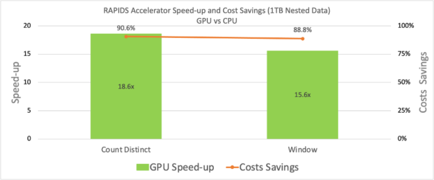
Currently, this jar supports training for the Principal Component Analysis algorithm. The ETL jar extended the input type support for Parquet and ORC. It now also provides users with the functionality to use HashAggregate, Sort, JoinSHJ and Join BHJ on nested data. In addition to support for nested datatypes a performance test was also run.
In the figure below, we show that the speed-up is observed for two queries using nested data type input. Some other interesting features that were added in v21.10 are, pos_explode, create_map and so on. Please refer to RAPIDS Accelerator for Apache Spark’s documentation for a detailed list of new features.
Figure 2: Microbenchmark Queries runtime for nested datatypes on Google Cloud Platform Dataproc Cluster: GPU vs CPU.
Profiling & qualification tool
In addition to the plug-in, multiple new features were also added to RAPIDS Accelerator for Apache Spark’s Qualification and Profiling tool. The Qualification tool can now report the different nested datatypes and write data formats present. It now also includes support for adding conjunction and disjunction filters, and filter based Regular Expressions and usernames.
The Qualifications tool is not the only one with new tricks: the Profiling tool now provides structured output format and support to scale and run a large number of event logs.
Community updates
We are excited to announce that we are in public preview on Azure and we welcome Azure users to try RAPIDS Accelerated for Apache Spark on Azure Synapse.
The upcoming versions will introduce support for 128-bit decimal datatype, inference support for the Principle Component Analysis algorithm and additional nested data type support for multi-level struct and maps.
In addition, lookout for MIG support for NVIDIA Ampere Architecture based GPUs (A100/A30) which can help improve throughput on running multiple spark jobs with A100. As always, we want to thank all of you for using RAPIDS Accelerator for Apache Spark and we look forward to hearing from you. Reach out to us on GitHub and let us know how we can continue to improve your experience using RAPIDS Accelerator on Apache Spark.
GeForce NOW is charging into the new year at full force. This GFN Thursday comes with the news that Genshin Impact, the popular open-world action role-playing game, will be coming to the cloud this year, arriving in a limited beta. Plus, this year’s CES announcements were packed with news for GeForce NOW. Battlefield 4: Premium Read article >
Practice machine learning operations and learn how to deploy your own machine learning models on a NVIDIA Triton GPU server.
Deploying a Model for Inference at Production Scale
A lot of love goes into building a machine-learning model. Challenges range from identifying the variables to predict to experimentation finding the best model architecture to sampling the correct training data. But, what good is the model if you can’t access it?
Enter the NVIDIA Triton Inference Server. NVIDIA Triton helps data scientists and system administrators turn the same machines you use to train your models into a web server for model prediction. While a GPU is not required, an NVIDIA Triton Inference Server can take advantage of multiple installed GPUs to quickly process large batches of requests.
NVIDIA Triton was created with Machine Learning Operations, or MLOps, in mind. MLOps is a relatively new field evolved from Developer Operations, or DevOps, to focus on scaling and maintaining machine-learning models in a production environment. NVIDIA Triton is equipped with features such as model versioning for easy rollbacks. It is also compatible with Prometheus to track and manage server metrics such as latency and request count.
Course Information
This course covers an introduction to MLOps coupled with hands-on practice with a live NVIDIA Triton Inference Server.
Learning objectives include:
Deploying neural networks from a variety of frameworks onto a live NVIDIA Triton Server.
Measuring GPU usage and other metrics with Prometheus.
Sending asynchronous requests to maximize throughput.
Upon completion, developers will be able to deploy their own models on an NVIDIA Triton Server.
Autonomous vehicles are born in the data center, which is why NVIDIA and Deloitte are delivering a strong foundation for developers to deploy robust self-driving technology. At CES this week, the companies detailed their collaboration, which is aimed at easing the biggest pain points in AV development. Deloitte, a leading global consulting firm, is pairing Read article >
After running the script “model_main_tf2.py”, I received the following error message:
-> INFO:tensorflow:Waiting for new checkpoint at models/my_ssd_resnet50_v1_fpn -> I1220 17:06:56.024288 140351537808192 checkpoint_utils.py:140] Waiting for new checkpoint at models/my_ssd_resnet50_v1_fpn -> INFO:tensorflow:Found new checkpoint at models/my_ssd_resnet50_v1_fpn/ckpt-2 -> I1220 17:06:56.024974 140351537808192 checkpoint_utils.py:149] Found new checkpoint at models/my_ssd_resnet50_v1_fpn/ckpt-2 -> 2021-12-20 17:06:56.098253: I tensorflow/compiler/mlir/mlir_graph_optimization_pass.cc:185] None of the MLIR Optimization Passes are enabled (registered 2) -> /home/ameisemuhammed/anaconda3/envs/tensorflow/lib/python3.9/site-packages/keras/backend.py:401: UserWarning: tf.keras.backend.set_learning_phase is deprecated and will be removed after 2020-10-11. To update it, simply pass a True/False value to the `training` argument of the `call` method of your layer or model. -> warnings.warn(‘`tf.keras.backend.set_learning_phase` is deprecated and ‘ -> 2021-12-20 17:07:08.993353: I tensorflow/stream_executor/cuda/cuda_dnn.cc:369] Loaded cuDNN version 8204 -> Traceback (most recent call last): -> File “/home/ameisemuhammed/TensorFlow/workspace/training_demo/model_main_tf2.py”, line 114, in <module> tf.compat.v1.app.run() -> File “/home/ameisemuhammed/anaconda3/envs/tensorflow/lib/python3.9/site-packages/tensorflow/python/platform/app.py”, line 40, in run _run(main=main, argv=argv, flags_parser=_parse_flags_tolerate_undef) -> File “/home/ameisemuhammed/anaconda3/envs/tensorflow/lib/python3.9/site-packages/absl/app.py”, line 303, in run _run_main(main, args) -> File “/home/ameisemuhammed/anaconda3/envs/tensorflow/lib/python3.9/site-packages/absl/app.py”, line 251, in _run_main sys.exit(main(argv)) -> File “/home/ameisemuhammed/TensorFlow/workspace/training_demo/model_main_tf2.py”, line 81, in main model_lib_v2.eval_continuously( -> File “/home/ameisemuhammed/anaconda3/envs/tensorflow/lib/python3.9/site-packages/object_detection/model_lib_v2.py”, line 1141, in eval_continuously optimizer.shadow_copy(detection_model) -> File “/home/ameisemuhammed/anaconda3/envs/tensorflow/lib/python3.9/site-packages/keras/optimizer_v2/optimizer_v2.py”, line 830, in getattribute raise e -> File “/home/ameisemuhammed/anaconda3/envs/tensorflow/lib/python3.9/site-packages/keras/optimizer_v2/optimizer_v2.py”, line 820, in getattribute return super(OptimizerV2, self).getattribute(name) -> AttributeError: ‘SGD’ object has no attribute ‘shadow_copy’“
What started as Nick Walton’s college hackathon project grew into AI Dungeon, a popular text adventure game with over 1.5 million users. Walton is the co-founder and CEO of Latitude, a Utah-based startup that uses AI to create unique gaming storylines. He spoke with NVIDIA AI Podcast host Noah Kravitz about how natural language processing Read article >
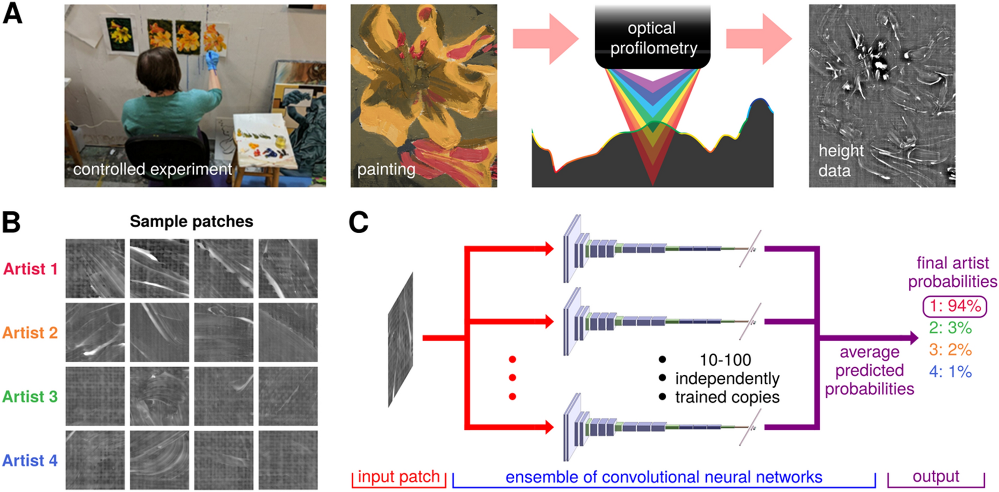
Researchers developed a new AI algorithm that can identify a painter based on brushstrokes, with precision down to a single bristle.
Spotting painting forgeries just became a bit easier with a newly developed AI tool that picks up style differences with precision down to a single paintbrush bristle. The research, from a team at Case Western Reserve University (CWRU), trained convolutional neural networks to learn and identify a painter based on the 3D topography of a painting. This work could help historians and art experts distinguish between artists in collaborative pieces, and find fraudulent copies.
There are several methods to authenticating antique paintings. Experts often evaluate the style and condition of materials and use scientific methods such as microscopic analysis, infrared spectroscopy, and reflectography.
However, these exhaustive methods are time-consuming and can result in errors. They also cannot identify multiple painters of one piece of art. According to the study, painters such as El Greco and Rembrandt often employed workshops of artists to paint parts of a canvas in the same style as their own, making individual contributions unclear.
While analyzing artwork with machine learning is a relatively new field, recent studies have focused on combining AI methods with high-resolution images of paintings to learn a painter’s style and identify an artist. The researchers hypothesized that 3D analysis could hold even more data than an image, where features such as brushwork patterns along with paint deposition and drying methods could serve as an artist’s unique fingerprint.
“3D topography is a new way for AI to ‘see’ a painting,” senior author Kenneth Singer, the Ambrose Swasey Professor of Physics at CWRU, said in a press release.
Extracting topographical data from a surface with an optical profiler, the researchers scanned 12 paintings of the same scene, painted with identical materials, but by four different artists. Sampling small square patches of the art, approximately 5 to 15 mm, the optical profiler detects and logs minute changes on a surface, which can be attributed to how someone holds and uses a paintbrush.
They then trained an ensemble of convolutional neural networks to find patterns in the small patches, sampling between 160 to 1,440 patches for each of the artists. Using NVIDIA GPUs with cuDNN-accelerated deep learning frameworks, the algorithm matches the samples back to a single painter.
The team tested the algorithm against 180 patches of an artist’s painting, matching the samples back to a painter at about 95% accuracy.
According to coauthor Michael Hinczewski, the Warren E. Rupp Associate Professor of Physics at CWRU, the ability to work with such small training sets is promising for later art historical applications with limited training datasets.
Figure 1: Overview of the data acquisition workflow and an ensemble of convolutional neural networks used to assign artist attribution probabilities to each patch. Credit: Ji, F., McMaster, M.S., Schwab, S. et al./Herit Sci
“Most of the other studies using AI for art attribution are focused on photos of entire paintings,” said Hinczewski. “We broke the painting down into virtual patches ranging from one-half millimeter to a few centimeters square. So we no longer even have information about the subject matter—but we can accurately predict who painted it from an individual patch. That’s amazing.”
Based on their findings the researchers view surface topography as an additional tool for attribution and forgery detection using an unbiased and quantitative analysis. In a collaboration with art conservation company Factum Arte based in Madrid, the team is working on artist workshop attribution and conservation studies on several works of the Spanish Renaissance painter El Greco.
The data and code associated with the research are available through GitHub. The work is a joint effort between researchers from the CWRU Department of Art History and Art, Cleveland Institute of Art, and the Cleveland Museum of Art.

 This post details the latest functionality of RAPIDS Accelerator for Apache Spark.
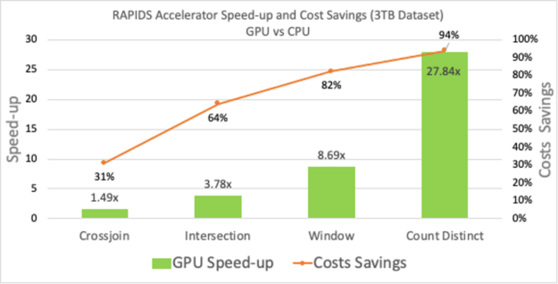
 Practice machine learning operations and learn how to deploy your own machine learning models on a NVIDIA Triton GPU server.


 Researchers developed a new AI algorithm that can identify a painter based on brushstrokes, with precision down to a single bristle.