Data Scientists role in producing AI related written content to be consumed by the public
Editor’s Note: If you’re interested sharing your data science and AI expertise, you can apply to write for our blog here.
Primarily the dual purpose of writing has been to preserve and transfer knowledge across communities, organizations, and so on. Writing within the machine-learning domain is used for the sole purposes mentioned. There are prominent individuals that have placed immense time and effort in advancing the frontier of machine learning and AI as a field. Coincidentally, a good number of these AI pioneers and experts write a lot.
This article includes individuals that have contributed to the wider field of AI in different shapes and forms, especially, emphasizing their written work. The contribution each individual has provided through the practice of writing AI-related content.
The essential takeaway from this article is that as Data Scientists it’s a requirement that we develop soft skills such as creative and critical thinking, alongside communication. Writing is an activity that cultivates the critical soft skills for Data Scientists.
AI Experts That Write
Andrej Karpathy
At the time of writing, Andrej Karpathy is Senior Director of AI at Tesla. Overseeing engineering and research efforts on bringing commercial autonomous vehicles to market, by using massive artificial neural networks trained with millions of image and video samples.
Andrej is a prominent writer. His work has featured in top publications such as Forbes, MIT Technology Review, Fast Company, and Business Insider. Specifically, I’ve been following Andrej’s writing through his Medium profile and his blog.
In my time as a Computer Vision student exploring the fundamentals of convolutional neural networks, Andrej’s Deep learning course at Stanford proved instrumental in gaining an understanding and intuition of the internal structure of a convolutional neural network. Specifically, the written content of the course explored details such as the distribution of parameters across the CNN, the operations of the different layers within the CNN architecture and the convolution operation that occurs between CNN’s filter parameters, and the values of an input image. Andrej uses his writing to present new ideas, explore the state of deep learning, and educate others.
Data Scientists are intermediaries between the world of numerical representations of data and project stakeholders, therefore the ability to interpret and convey derived understanding from datasets is essential to Data Scientists. Writing is one means of communication that equips Data scientists with the capability to convey and present ideas, patterns, and learning from data. Andrej’s writing is a clear example of how this is done. He provides a clear and concise-written explanation of neural network architecture, data preparation processes and many more.
Kai-Fu Lee
Kai-Fu Lee is an AI and Data Science Expert. He has contributed significantly to AI through his work at Google, Microsoft, Apple, and other organizations.
He’s currently CEO of Sinovation Ventures. Kai-Fu has been making significant contributions to AI research by applying Artificial Intelligence in video analysis, computer vision, pattern recognition, and so on. Furthermore, Kai-Fu Lee has written books exploring the global players of AI and the future utilization and impact of AI in his book AI Superpowers and AI 2041.
Through his writing, Kai-Fu Lee dissects the strategies of nations and entities that operate abundantly within the AI domain. The communication of decisions, mindset, and national efforts that drive the AI superpowers of today is crucial to the developing nations seeking to fast-track the development of AI technologies.
However, Kai-Fu Lee also conveys the potential disadvantages that the advancement of AI technologies can have on societies and individuals through his writing as well. By reading Kai-Fu Lee’s written contents, I’ve been able to understand how deep learning and predictive models can affect daily human lives when their usability is projected into imaginative future scenarios that touch on societal issues such as bias, poverty, discrimination, inequality, and so on.
The “dangers of AI” is a discourse that’s held more frequently as the adoption of AI technology and data-fueled algorithms become commonplace within our mobile devices, appliances, and processes. Data Scientists are ushering in the future one model at a time and it’s our responsibility to ensure that. We are able to communicate the fact that we conduct an in-depth cost-benefit analysis of technologies before they are integrated into society. These considerations put the mind of consumers at ease, by ensuring that the positive and negative impact of AI technology is not just afterthoughts to Data Scientists.
An effective method of communicating the previously mentioned considerations for Data Scientists is through writing. There’s effectiveness in writing a post or two explaining the data source, network architectures, algorithms, and extrapolated future utilization of AI applications or predictive models based on current utilization. A Data Scientist that covers these steps as part of their process establishes a sense of accountability and trust within product consumers and largely, the community.
Francois Chollet
TensorFlow and Keras are two primary libraries that are used extensively within data science and machine-learning projects. If you use any of these libraries, then Francois Chollet is probably an individual within AI you’ve come across.
Francois Chollet is an AI researcher that currently works as a Software Engineer at Google. He’s recognized as the creator of the deep-learning library Keras and also a prominent contributor to the TensorFlow library. And no surprise here, he writes.
Through his writing, Francois has expressed his thoughts on concerns, predictions, and limitations of AI. The impact of Francois writing on me as a machine-learning practitioner comes from his essays on software engineering topics, more specifically: API design and software development processes. Through his writing, Francois has educated hundreds of thousands on the topic of practical deep learning and utilization of the Python programming language for machine-learning tasks, through his infamous book Deep Learning With Python.
Through writing Data Scientists have the opportunity to enforce best practices in software development and data science processes among team members, or organizations.
Conclusion
Academic institutions covering Data Science should have writing within the course curriculum. The cultivation of writing as a habit through the years in academia proves beneficial in professional roles.
Professional Data Scientists should expand their craft by adopting writing as an integral aspect of communication of ideas, techniques, and concepts. As pointed out through the work of the AI experts mentioned in this article, written work produced can be in the form of essays, blogs, articles, and so on. Even interacting with peers and engaging in discourse on platforms such as LinkedIn or Twitter can be beneficial for Data Science professionals.
Novice Data Scientists often ask what methods can be adopted to improve skills, knowledge, and confidence, unsurprisingly the answer to that is also writing. Writing enables the expression of ideas in a structured manner that is difficult to convey through other communicative methods. Writing also serves as a method to reinforce learning.
This post is a fantastic resource of inspiration for Data Scientists looking for ideas, and if you’re feeling inspired, read this article about different sorts of writing in the field of machine learning.


 Learn about the optimizations and techniques used across the full stack in the NVIDIA AI platform that led to a record-setting performance in MLPerf HPC v1.0.
 v1.0 HPC Closed Strong & Weak Scaling – Result retrieved from
  Learn more about the many ways scientists are applying advancements in Million-X computing and solving global challenges.


 Meet The Spaghetti Detective, an AI-based failure-detection tool for 3D printer remote management and monitoring.
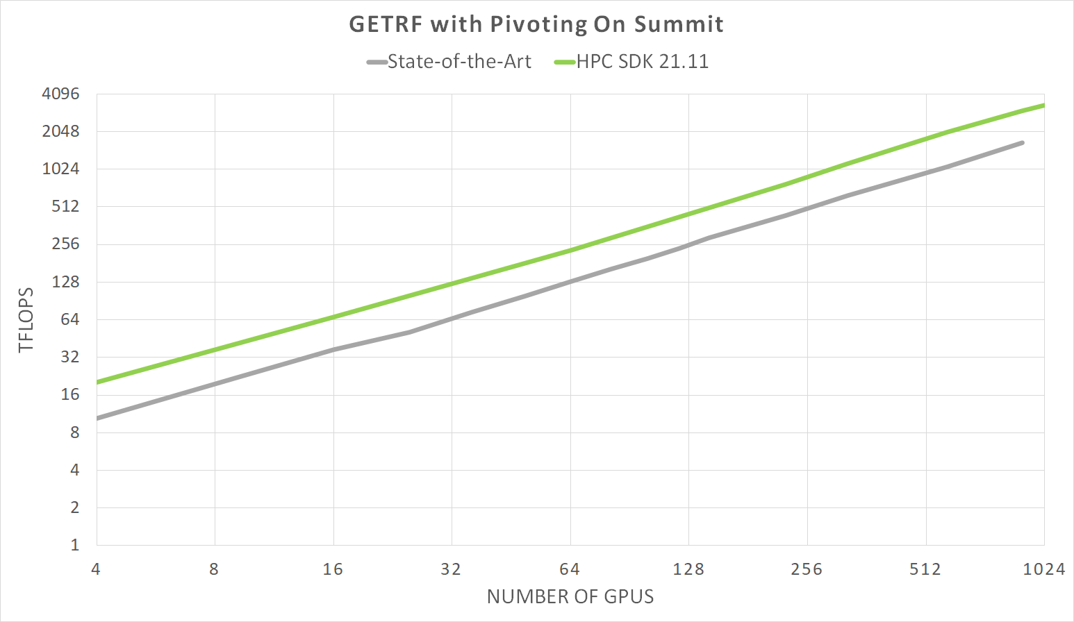
 The latest NVIDIA HPC SDK includes a variety of tools to maximize developer productivity, as well as the performance and portability of HPC applications.