Learn how AI is transforming the retail industry through enabling intelligent stores, omnichannel management, and automated supply chains.
Global retailers and suppliers are faced with navigating rapidly changing consumer demand, behavior, and expectations. These changes are driving uncertainty in forecasting and putting pressure on global supply chains as well as omni-channel and store operations. Real-time agility is required to navigate the rapidly evolving challenges for the retail industry.
Artificial intelligence offers a powerful solution for retailers to rapidly and more accurately forecast daily demand and automate supply chain logistics. This has a major impact on in-store supply and last-mile delivery cost challenges, while meeting consumer expectations on delivery timelines. For online shoppers, AI is helping create personalized shopping journeys and product recommendations. In-store, retailers are using AI to reduce shrinkage and stockout, while creating frictionless experiences and ensuring the health and safety of employees and shoppers.
The financial opportunity is significant across the $26 trillion retail industry, which historically has averaged a 2% net profit margin. An estimated 3X increase in profit margin with AI-enabled solutions would lead to over a $1 trillion increase in annual revenue for retailers, according to analysis by the McKinsey Global Institute. From customer engagement, to operational agility, to seamless omnichannel management, AI at the edge is transforming retail.
Retailers Adopt AI for Improved In-Store Experiences, Less Shrinkage
Retailers are leveraging AI at the edge to analyze data from in-store cameras and sensors, and create intelligent stores. One application alerts store associates when shelf inventory levels are low, reducing the impact of stockout. Another is decreasing shrinkage—the loss of inventory from theft, errors, fraud, waste, and damage—which costs the industry an estimated $100 billion per year globally. AI helps retailers protect their assets with store analytics that monitor points-of-sale and floor merchandise to prevent ticket switching, misscans, and shoplifting.
Deep North, a computer vision startup, uses intelligent video analytics to power in-store analytics, providing insights to customer traffic and heatmaps, determining dwell times, queue/wait times, conversion metrics, demographics, and more. These insights help retailers improve inventory planning, store layout and merchandising, and improve the customer experience and conversion.
Frictionless store concepts are being tested where shoppers can skip the checkout lines entirely and be automatically billed for their purchases. AiFi is a leader in these AI-enabled autonomous stores from nano stores to full-sized grocery chains. These “grab-and-go” stores are rising in popularity and locations are projected to expand 4X in the next 3 years.
Figure 1. AiFi provides autonomous shopping solutions leveraging computer vision powered by NVIDIA Metropolis for in-store analytics and the NVIDIA EGX platform for AI at the edge.
AI Personalizes Online Shopping
Personalized experiences are critical in ecommerce, which can account for as much as 30% of revenue for the world’s largest retailers. Underlying ecommerce are sophisticated recommender systems (RecSys). GPU-powered machine learning and deep learning enable recommenders by learning how customers shop, personalizing their shopping experience, and finding related items that shoppers are most likely to purchase. NVIDIA has deep domain expertise with our data science teams winning three global RecSys competitions in 5 months.
To support the online personalization and recommendations, global retailers are using AI to automatically generate metadata for new items listed in their vast digital catalogs. With up to millions of new products to onboard, comprehensively and accurately labeling and describing every product is a daunting task. AI quickly produces accurate, comprehensive, and engaging product content that a RecSys engine uses to provide personalized recommendations that attract a shopper’s interest.
Visual search is a key trend for retailers to provide a customer-centric experience with product search and discovery. Clarifai, a startup and NVIDIA Inception member, uses computer vision and AI to deliver more relevant search results and hyperpersonalized product recommendations quickly. With “snap-and-search” capabilities, shoppers are able to take a photo of a product they’re interested in with their mobile device and automatically have the photo matched to a product catalog. Related products to complete their desired outfit, room, or other look are also shared.
Smart virtual assistants, used by hundreds of millions of users each month, are also driving growth in ecommerce. Retailers are looking to improve the digital customer experience by introducing voice ordering to replace text-based searches with voice commands. With voice ordering, shoppers can easily search for items, ask for product information, and place online orders using smart speakers or other intelligent mobile devices.
Creating a Resilient Global Supply Chain
AI empowers retailers to create more resilient supply chains that respond quickly to changing consumer demand and effectively manage inventory distribution.
Walmart, for example, uses AI to run accurate daily forecasts of millions of item-to-store combinations across thousands of stores in the United States. Built on open-source data processing and machine learning libraries, this AI-powered platform enabled Walmart to get the right products to the right stores more efficiently, react in real time to shopper trends, and realize inventory cost savings at scale.
In smart warehouses, AI improves operational efficiency and throughput with customer orders automatically picked, packed, and shipped by robots. These robots use edge computing and intelligent video analytics to identify, position, and sort packages while adjusting the speed of conveyor belts to minimize product damage and machine downtime.
KION Group simplifies the deployment and management of AI at the edge— including autonomous forklifts and pick-and-place robotics—across thousands of retail distribution centers.
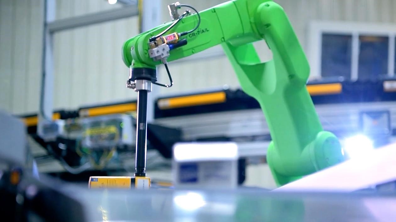
Figure 2. KION uses pick-and-place robots in its intelligent warehouses with AI deployed at the edge.
AI delivers end-to-end visibility that combines data from GPS, weather, traffic, and construction to determine optimal shipping routes. This can significantly reduce overhead costs for last-mile delivery associated with fuel, transportation, and delivery personnel—and can provide more accurate delivery windows that enhance customer service and create more satisfied shoppers.
Future of Edge Computing in Retail and Beyond
Billions of connected sensors are coming online in retail stores, city streets, hospitals, warehouses, and more. By deploying and managing scalable, secure AI at the edge, enterprises can turn this data into faster insights and more robust services and applications.
BlueField-2 offers protection, while delivering high security, integrity, and reliability for the new hybrid cloud era.
Data Processing Units, or DPUs, are the new foundation for a comprehensive and innovative security offering. The hyperscale giants and telecom providers have adopted this strategy for building and securing highly efficient cloud data centers, and it’s now available for enterprise customers. This strategy has revolutionized the approach to minimize risks and enforce security policies inside the data center.
A DPU is an integrated system on a chip (SOC) that combines high-performance CPU, network interface, and data center function accelerators into a single ASIC. DPUs utilize programmable hardware to offload and accelerate inline security services at line-rate.
BlueField DPU
The NVIDIA® BlueField®-2 DPU provides the first line of defense against attacks. Internal attacks that try to infiltrate the data center are prevented through an isolated, secure boot process and secure firmware updates. Aimed at accelerating security throughout the data center, DPUs are capable of filtering packets in support of next-generation firewalls and intrusion detection/prevention systems. A DPU can detect, block, and protect sensitive assets and data from threats.
The design offers built-in functional isolation to protect individual workloads and provide flexible control and visibility at the server level, reducing risk, and increasing efficiency. The isolation enables software agents and applications to run securely on the DPU, irrespective of the rest of the system.
Isolated from the host, and leveraging unique hardware capabilities, the DPU can deliver better security by reducing the attack surface and bolstering individual workload isolation—providing additional protection to reduce risks and simplify security management policies.
Furthermore, DPUs offload and accelerate cryptographic operations and offer encryption of data at rest or in motion. Freeing the host CPU to run critical applications, and being isolated from the application domain, keeps the cryptographic keys secure from a potentially compromised host.
The Changing Role of Firewall Security
The adoption of a cloud compute model calls for intelligent security solutions capable of delivering maximum performance and agility. In the age of hybrid cloud and virtualized computing, security functions have transformed. They are being deployed within every host to provide strict policy enforcement, as well as visibility into possible attacks.
Previously, protection within the host required running a software security solution or VM appliance, which was slow and consumed CPU resources. As new technology and bandwidth requirements increase, host-based protection now requires hardware performance at line-rate.
BlueField-2 DPU can be used as such a device to filter traffic traveling between computers. NVIDIA DPUs employ powerful hardware and software networking components that are programmable, with a configurable set of rules to inspect all traffic traversing the connection at line-rate. When combined with perimeter security solutions, a DPU can extend security to include host-based protection.
The DPU can be used as a platform that sits at the ingress and egress points of each host, adding a new layer where it’s needed most—at the computing edge. Together, they better protect against malicious threats to company assets and resources.
Software-based firewalls also place an additional burden on the CPU, reducing available computing resources for application processing and decreasing the number of VM, applications, and services that can run on a single host. BlueField-2 DPU security platform, with a software security stack, offloads security services from the host, freeing CPU cycles for applications running on host resources.
Micro-Segmentation
The complexity of security increases with the use of computing and network virtualization technologies. Micro-segmentation is a network security technique in virtualized environments that logically divides a data center into distinct individual security segments at the workload level. At this low-level, security controls can be defined, and security services delivered for each unique segment. BlueField-2 provides a platform for hosting micro-segmentation and network connection tracking services for flow-based network analytics and application-level security for traffic inside the data center.
The DPU can run a security software stack, leaving no impact on servers or hindering application performance. This hardware-accelerated solution includes security policies and enforcement capabilities at wire speed and is fully isolated from the application workloads themselves.
The decade-old approach of perimeter security defense has reached a tipping point of performance limitations and operational complexities. A new holistic approach to security is needed for enterprises to achieve robust protection. Enterprise data centers are evolving and following the lead of hyperscale and public cloud providers with CDI and should also adopt their similar tactics for network security. BlueField-2 can offer protection for all types of workloads against current and future threats, and can deliver the highest security, integrity, and reliability for the new hybrid cloud era.
As the cybersecurity landscape grows in complexity, security experts continue to turn to NVIDIA BlueField-2 as a platform to provide advanced security features.
Our security experts are here to help answer questions about how BlueField-2 can augment and expand your security solution. If you’re a security architect or product manager at a cybersecurity company, contact us.
Simulations are pervasive in every domain of science and engineering, but they often have constraints such as large computational times, limited compute resources, tedious manual setup efforts, and the need for technical expertise. Neural networks not only accelerate simulations done by traditional solvers, but also simplify simulation setup and solve problems not addressable by traditional … Continued
Simulations are pervasive in every domain of science and engineering, but they often have constraints such as large computational times, limited compute resources, tedious manual setup efforts, and the need for technical expertise. Neural networks not only accelerate simulations done by traditional solvers, but also simplify simulation setup and solve problems not addressable by traditional solvers.
NVIDIA SimNet is a physics-informed neural network (PINN) toolkit for engineers, scientists, students, and researchers who are getting started with AI-driven physics simulations. You may also be looking to leverage a powerful, existing framework to implement your domain knowledge and solve complex nonlinear physics problems with real-world applications.
A success story of SimNet’s application today is in the use of hybrid PINNs for digital twins in prognosis and health management. This effort was led by Prof. Felipe Viana, an assistant professor at the University of Central Florida. He leads the group’s research in state-of-the-art probabilistic methods fusing physics-based domain knowledge and multidisciplinary analysis and optimization with applications in design, diagnostics, and prognostics.
Aircraft use case study
Maintenance of engineering assets and industrial equipment (such as aircraft, jet engines, wind turbines, and so on) is critical for safety as well as enhanced profitability in the services and warranties of these assets. Effective preventive maintenance requires the knowledge of the various operating parameters and their impact on the wear and tear of equipment. Simulations, advanced analytics, and deep learning algorithms enable the predictive modeling of complex systems and their operating environment.
Unfortunately, building models that estimate residual useful life for such equipment in large fleets is daunting. This is due to factors such as duty cycle variations, harsh environments, inadequate maintenance, and mass production problems that cause discrepancies between designed and observed component lives.
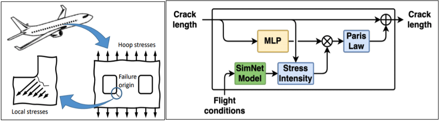
In this research project, Prof. Viana and his team of researchers built predictive models for fatigue crack growth prognosis on aircraft window panels (Figure 1), where models were trained using historical flight records (origin and destination airports, cruise altitude, and so on) and limited inspection observations (such as the crack length data for only a portion of the fleet, and so on). When the model was built and validated, it was then applied in a fleet of 500 aircraft to analyze the success of the model on larger data sets. Such predictive models are also called digital twin models and they have been increasingly used in prognosis and health management applications of industrial equipment.
Figure 1. Fatigue crack growth at fuselage panel
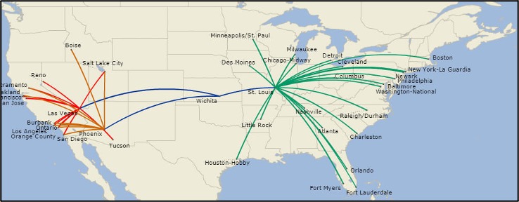
Based on literature and freely available data, synthetic data for a representative fleet of 500 narrow-body aircraft was created. The fleet is equally divided into 10 route structures (Figure 2). Each aircraft flies an average of five flights per day.
Figure 2. Aircraft routes
After four years of operation, the fleet starts being inspected. At this point, consider a case in which after inspecting 25 aircraft, the operator finds that some exhibit fatigue cracks at the corner of a given window. These cracks happen to be larger than anticipated. From a scientific standpoint, this poses the following challenge: if predictions were wrong due to model assumptions, is there a way to correct that?
The business implication is straightforward. When such a discrepancy is observed, operators must decide which aircraft to inspect next.
Assume that you have available the flight data from the fleet for the past four years. The hoop stresses that govern the fatigue crack growth are a function of the aircraft cabin pressure differential, which is a function of cruise altitude. The purely physics-based model assumes the local geometry correction factor F = 1.122. In reality, that is ultimately a function of the crack length. The digital twin for this component must be predictive and aircraft-specific, in addition to being computationally efficient.
There are two main challenges. First, the data is highly unbalanced. For the aircraft fleet that was being analyzed, there were only 182,500 input points and only 25 output points. Building purely machine learning models under such circumstance is extremely hard.
Second, while the conventional physics-based models maybe accurate, they often entail engineering assumptions regarding loading conditions. Considering that the sample size for this problem includes a fleet of 500 aircraft, these simulations must be done a few million times.
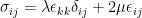
To overcome these challenges, Prof. Viana and team developed a novel hybrid physics-informed neural network model. Figure 3 shows where they performed cumulative damage accumulation based on recurrent neural networks merging physics-informed and data-driven layers.
Figure 3. Physics informed kernels within the recurrent network
Full-fledged finite element analysis configured for crack growth simulation is extremely expensive. Therefore, it is simply not feasible for digital twin applications. This is true even if we were to run simulations for hundreds of aircraft many times over, as we optimized inspections and decided how to swap routes for a few aircraft. A parameterized physics-driven AI model is constructed in SimNet that satisfies the governing laws of linear elasticity, as follows:
Here, is the Cauchy stress tensor, is the Kronecker delta function and is the strain tensor. The inputs to this parameterized model are the loading condition (the hoop stresses) and the spatial coordinates of batches of a point cloud within the computational domain. The outputs are the stresses and displacements. The network architecture consists of a Fourier feature encoding layer followed by several fully connected layers.
Unlike the traditional data-driven models, no training data is used here. Instead, the loss functions are augmented by the linear elasticity laws, and the required second-order derivatives are computed using automatic differentiation. Initial and boundary conditions are also imposed as soft constraints to fully specify the physical system. Several techniques are used to enhance the accuracy and convergence speed of the model, such as network weight normalization, signed distance loss weighting, differential equation normalization and nondimensionalization, and XLA kernel fusion.
After a single training, this parameterized model provides instantaneous prediction of cyclic stresses for a variety of different loading conditions. This instantaneous prediction is critical in digital-twin applications where real-time predictions are needed. However, traditional solvers can only solve for one configuration at a time. Moreover, data-driven, surrogate-based approaches suffer from interpolation error and the predictions may not satisfy the governing laws.
For this trained parameterized model, several SimNet predictions are validated against a commercial solver, showing a close agreement with a difference of less than 5% in the maximum Von Mises stresses. Training of this model was performed on a single V100 GPU. SimNet also offers scalable performance for multi-GPU and multi-node implementation with TF32 support for accelerated convergence.
In Prof. Viana’s model, engineers and scientists can use physics-informed layers to model well-understood phenomena. This might include mechanical stress calculations to estimate the damage accumulation with Paris law fatigue increment block. Another example would be using data-driven layers to model poorly characterized parts such as corrections in stress intensity due to geometry of crack. This is where hybrid models can help estimate fatigue crack growth on fuselage panels with window cutouts.
In Figure 4, the “before training” curve uses purely physics-based models. These are obtained through numerical integration of Paris law using linear elasticity in the calculation of cyclic stresses:
: number of cycles
and : material properties (obtained through coupon tests)
: cyclic stresses (for example, from finite element models)
In Figure 4, the “after training” curve uses the hybrid model where the MLP layer in the RNN cell compensates for missing physics (adjusting predictions without violating the physics).
Figure 4. Predicted compared to actual crack length at inspected aircraft
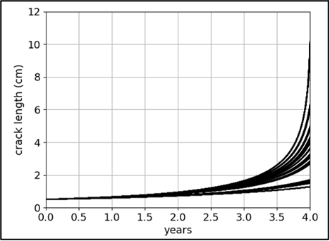
After the hybrid model is trained, we use it to predict crack length histories for the entire fleet of 500 aircraft. The 500 pressure differential time series amount for more than 3.5M data points. The hybrid cumulative damage recurrent neural network, using SimNet for stress calculations, predicts the crack length histories in 5 years. The results are illustrated in Figure 5. This enables the operators to prioritize which aircraft will be brought for inspection or swapping aircraft of different route structures.
Figure 5. Crack length history over the years
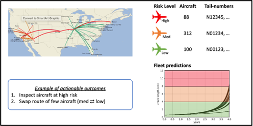
Operators could use the hybrid model to analyze the entire fleet. The results dashboard could visualize the most aggressive route structures in terms of cumulative damage rates; number of aircraft at high, medium, or low risk levels; as well which tail numbers are in which buckets (Figure 6).
Figure 6. Fleet dashboard
In terms of actionable outcomes, operators could use the hybrid model to decide which aircraft should be brought for inspection next. They could swap aircraft between routes so that damage accumulation is mitigated while inspections are performed.
This framework handles highly unbalanced datasets formed by few output observations and data lakes containing time series used as inputs. GPU computing enables scaling up computations for fleets of hundreds of aircraft, keeping training under a few hours and inference under a few seconds.
Prof. Viana’s application’s implementation has been done in TensorFlow v2.3 using the Python APIs on various NVIDIA GPUs. Depending on the application and computing needs, you can use high-performance GPU-based clusters, a smaller Linux server with few GPUs, or even the NVIDIA Jetson. For this study, we used a Linux server with two Intel Xeon Processor E5-2683 and two NVIDIA P100 GPUs.
Next steps
In the future, Prof. Viana and his team plan on expanding the use of SimNet in their hybrid PINNs for cumulative damage by tackling even more complex applications where loading and deformation are highly nonlinear and potentially involve multiphysics. Given the flexibility of the approach, he hopes to expand the applications to other industries besides civil aviation and failure modes, such as corrosion and oxidation.
Prof. Viana elaborated on his experience. “SimNet’s accuracy is comparable to other computational mechanics software. However, its computational efficiency, quick turnaround time, and easy integration with existing machine learning frameworks makes it our choice of toolkit for our simulation needs. With SimNet, we scaled our predictive model to a fleet of 500 aircraft and get predictions in less than 10 seconds. If we were to perform the same computations using high-fidelity finite element models, we could be talking about a few days to a week. As a research institution, we see SimNet as a tool of the future where it unlocks possibilities and enables us to explore modeling approaches that were not possible before.”
For more information, see the following resources:
To ask questions about Prof. Viana’s work and see what others are doing with SimNet toolkit, join the SimNet forum. For more information about SimNet’s features and to download the SimNet toolkit, see NVIDIA SimNet.
Speedy diagnoses are critical, especially when a loved one seems to be slowly losing their cognitive abilities. Researchers from the Kaunas University of Technology in Lithuania report they’ve developed a deep learning-based method able to predict the possible onset of Alzheimer’s disease from brain images with an accuracy of over 99 percent. The impact of Read article >
The NVIDIA Clara AGX development kit with the us4R ultrasound development system makes it possible to quickly develop and test a real-time AI processing system for ultrasound imaging.
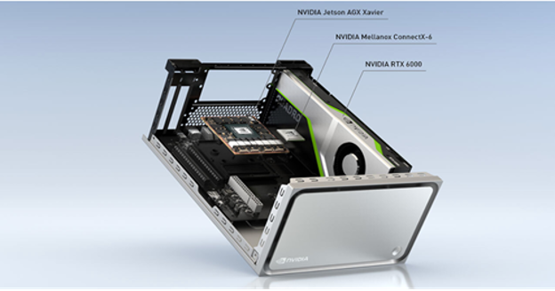
The NVIDIA Clara AGX development kit with the us4R ultrasound development system makes it possible to quickly develop and test a real-time AI processing system for ultrasound imaging. The Clara AGX development kit has an Arm CPU and high-performance RTX 6000 GPU. The us4R teamwork provides ultrasound system designers with the ability to develop, prototype, and test end-to-end software-defined ultrasound systems. Clara AGX is launching the era of software-defined medical instruments with reconfigurable pipelines without changes to the hardware.
The us4us hardware and SDK provide an end-to-end ultrasound algorithm development and RF processing platform, while the high-end Clara AGX GPU enables real-time deep learning and AI image reconstruction and inferencing. With this approach, the whole systems engineering team benefits: beamforming experts can create optimal beam strategies, and AI experts can design and deploy the next generation of real-time algorithms.
This combined hardware and software platform democratizes ultrasound development for both research labs and commercial vendors to develop novel features. No longer are massive capital budgets required to design, prototype, and test functional hardware. Each stage of the device pipeline can be modified. Data acquisition, data processing, image reconstruction, image processing, AI analysis, and visualization are all defined in software and executed in real time with low latency performance. The system is completely configurable and can create new RF transmission waveforms and beamforming algorithms using AI or traditional approaches.
With ultrafast, low latency end-to-end data transfer is possible with NVIDIA ConnectX-6 SmartNIC 100Gb/s ethernet and RDMA data transfer to the GPU. The NVIDIA supercharged GPU can run circles around existing legacy premium-cost systems. It enables improved signal-to-noise, real-time processing of highly advanced and complex algorithms in image reconstruction, denoising, and pipelines.
The GPU has enough headroom for multiple real-time clinical inferencing predictions to run simultaneously, including measurement, operator guidance, image interpretation, tissue and organ identification, advanced visualization, and clinical overlays.
Commercialization of clinical applications of the Clara AGX hardware will be available with medical-grade hardware from third party vendors in a compact and energy-efficient CPU+GPU SoC form-factor similar to that in self-driving automotive applications.
The Clara AGX development kit is a high-end performance workstation built with development of medical applications in mind. The system includes an NVIDIA RTX 6000 GPU, delivering 200+ INT8 AI TOPs and 16.3 FP32 TFLOPS at peak performance, with 24 GB of VRAM. This leaves plenty of headroom for running multiple models. High-bandwidth I/O communication with sensors is possible with the 100G Ethernet Mellanox ConnectX-6 network interface card (NIC).
NVIDIA partners are currently using the Clara AGX development kit to develop ultrasound, endoscopy, and genomics applications.
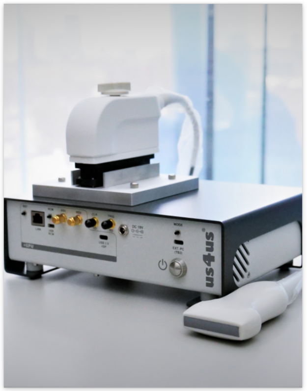
Advanced us4R with up to 1024 TX / 256 RX channels
A portable us4R-lite with 256 TX / 64 RX channels
Both use a PCIe streaming architecture for low-latency data transfer and GPU for scalable processing of raw ultrasound echo signals. The us4OEM ultrasound frontend modules support 128TX/32RX analog channels and high throughput 3GB/s, PCIe Gen3 x4 data interface (Figure 2).
Figure 3. Us4r-lite and Clara AGX platform
End-to-end, software-defined ultrasound design
The ARRUS package is an SDK for the us4R that provides a high-level hardware abstraction layer enabling systems programming in Python, C++, or MATLAB. The hardware programming is performed by defining RF module including the following:
Active transmit (TX) probe elements
Transmission parameters, such as TX voltage, TX waveform, and TX delays
Receive (RX) aperture and acquisition parameters such as gain, filters, and time-gain compensation
Commonly used TX/RX sequences, such as classical linear scanning, plane wave imaging (PWI) and synthetic transmit aperture (STA) are preconfigured and can be quickly implemented. Custom sequences are configured with user-defined, low-level parameters like TX/RX apertures mask and TX delays.
The ARRUS package also includes a Python implementation of many standard ultrasound processing algorithms for image reconstruction, including raw RF data, RF data preprocessing (data filtering, quadrature demodulation, and so on), beamforming (PWI, STA, and classical schemes), and post-processing of B-mode images.
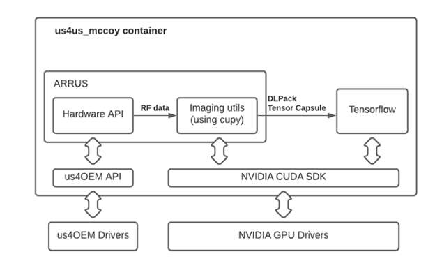
These algorithms are building blocks used to construct an arbitrary imaging pipeline that can handle the RF data stream produced by the us4R system. GPU accelerated numerical routines are provided by cuPy. DLPack specifies a common in-memory Tensor structure that enables data sharing between machine learning frameworks and GPU processing libraries, while using RDMA no additional overhead is required to copy data between them. The DLPack interface provides access to predefined or user-developed deep learning models in TensorFlow, PyTorch, Chainer, and MXNet.
Figure 4. NGC container software schematic for this release
US4US ultrasound demo
By combining the software and hardware stack, you can quickly implement an ultrasound workflow with configurable parameters in less than one page of easy-to-read Python code. In this section, we show you how to use the ARRUS APIs, a us4R-lite platform, and the Clara AGX DevKit to create your own ultrasound imaging pipeline in minutes.
The following code example should work with the proper environment. However, we recommend using the Docker container available directly through NGC. There is an interactive Jupyter notebook available to help guide you through this demo in the container at /us4us_examples/mimicknet-example.ipynb.
Start by importing the relevant libraries, including ARRUS, Numpy, TensorFlow, and CuPy:
# Imports for ARRUS, Numpy, TensorFlow and CuPy
 import arrus
 import arrus.session
 import arrus.utils.imaging
 import arrus.utils.us4r
 import numpy as np
 from arrus.ops.us4r import (Scheme, Pulse, DataBufferSpec)
 from arrus.utils.imaging import ( Pipeline, Transpose,  BandpassFilter,  Decimation,  QuadratureDemodulation, EnvelopeDetection, LogCompression, Enqueue,  RxBeamformingImg,  ReconstructLri,  Sum,  Lambda,  Squeeze)
 from arrus.ops.imaging import ( PwiSequence )
 from arrus.utils.us4r import ( RemapToLogicalOrder )
 from arrus.utils.gui import ( Display2D )
 from utilities import RunForDlPackCapsule, Reshape
 import TensorFlow as tf
 import cupy as cp
Next, instantiate the PWI Tx and Rx sequences. You define the parameters for the data that you’re pulling from the US4US Ultrasound system in the PwiSequence function.
After defining the sequence, load the deep learning model parameters. For this, you have two different deep neural networks options for improving B-mode image output quality, both available for download through NGC.
The NN_Bmode model, from researchers at Stanford, produces despeckled images using a neural network from beamformed low-resolution images (LRI). The LRI is created after a single synthetic aperture transmission; in this case, a single plane wave insonification. A sequence of LRIs can be compounded into a high-resolution image (HRI) by coherently summing them together.
The generative adversarial networks (GANs) model is used to imitate B-mode image post-processing found in commercial ultrasound systems. This algorithm uses the standard delay-and-sum (DAS) reconstruction and B-mode post-processing pipeline with the MimickNet CycleGAN. For more information, see MimickNet, Mimicking Clinical Image Post-Processing Under Black-Box Constraints.
For this example, you load the MimickNet CycleGAN. In addition to loading the weights, you are implementing simple normalize and mimicknet_predict wrapper functions required when you implement the scheme definition in the next step.
# Load MimickNet model weights
 model = tf.keras.models.load_model(model_weights)
 model.predict(np.zeros((1, z_size, x_size, 1), dtype=np.float32))

 def normalize(img):
     data = img-cp.min(img)
     data = data/cp.max(data)
     return data

 def mimicknet_predict(capsule):
     data = tf.experimental.dlpack.from_dlpack(capsule)
     result = model.predict_on_batch(data)

# Compensate a large variance of the image mean brightness.
     result = result-np.mean(result)
     result = result-np.min(result)
     result = result/np.max(result)
     return result
You can put all of the pieces together using the Scheme function. The Scheme function takes parameters for the tx/rx sequence definition: an output data buffer, the ultrasound device work mode, and a data processing pipeline. These parameters define the workflow for data acquisition, data processing, and displaying the inference results.
The following code example shows the Scheme definition, which includes the sequence, MimickNet preprocessing, and inference wrapper function defined earlier. The placement parameter indicates that the processing pipeline runs on GPU:0, which provides GPU acceleration on the Clara AGX Dev Kit.
Your device now displays the results of the ultrasound imaging pipeline. You can also easily modify this pipeline to implement your own state-of-the-art deep learning algorithms. Figure 5 shows the example output from the demo comparing a conventional delay and sum algorithm (left) and the MimickNet model (right).
Figure 5. Scan of an ultrasound phantom using standard delay and sum (left), NN_Bmode despeckling neural network (middle), MimickNet CycleGAN network (right)
Clara AGX is launching the era of software-defined medical instruments with re-configurable pipelines without changes to the hardware. Connecting the Clara AGX development kit with the us4R ultrasound development system creates a combination that helps you develop a real-time AI processing system easily and quickly. With the high performance of an RTX 6000 GPU and an Arm CPU, you get the best of the embedded hardware ecosystem to develop your own state-of-the-art, task-specific algorithms.
For more information about the us4R-lite system, contact us4us. The Clara AGX Developer Kit is currently available exclusively for members of the NVIDIA Clara Developer Partner Program.
Posted by Katrin Tomanek, Software Engineer and Bob MacDonald, Technical Program Manager, Google Research
Speech impairments affect millions of people, with underlying causes ranging from neurological or genetic conditions to physical impairment, brain damage or hearing loss. Similarly, the resulting speech patterns are diverse, including stuttering, dysarthria, apraxia, etc., and can have a detrimental impact on self-expression, participation in society and access to voice-enabled technologies. Automatic speech recognition (ASR) technologies have the potential to help individuals with such speech impairments by improving access to dictation and home automation and by enhancing communication. However, while the increased computational power of deep learning systems and the availability of large training datasets has improved the accuracy of ASR systems, their performance is still insufficient for many people with speech disorders, rendering the technology unusable for many of the speakers who could benefit the most.
Impaired Speech Data Collection Since 2019, speakers with speech impairments of varying degrees of severity across a variety of conditions have provided voice samples to support Project Euphonia’s research mission. This effort has grown Euphonia’s corpus to over 1 million utterances, comprising over 1400 hours from 1330 speakers (as of August 2021).
To simplify the data collection, participants used an at-home recording system on their personal hardware (laptop or phone, with and without headphones), instead of an idealized lab-based setting that would collect studio quality recordings.
To reduce transcription cost, while still maintaining high transcript conformity, we prioritized scripted speech. Participants read prompts shown on a browser-based recording tool. Phrase prompts covered use-cases like home automation (“Turn on the TV.”), caregiver conversations (“I am hungry.”) and informal conversations (“How are you doing? Did you have a nice day?”). Most participants received a list of 1500 phrases, which included 1100 unique phrases along with 100 phrases that were each repeated four more times.
Speech professionals conducted a comprehensive auditory-perceptual speech assessment while listening to a subset of utterances for every speaker providing the following speaker-level metadata: speech disorder type (e.g., stuttering, dysarthria, apraxia), rating of 24 features of abnormal speech (e.g., hypernasality, articulatory imprecision, dysprosody), as well as recording quality assessments of both technical (e.g., signal dropouts, segmentation problems) and acoustic (e.g., environmental noise, secondary speaker crosstalk) features.
Personalized ASR Models This expanded impaired speech dataset is the foundation of our new approach to personalized ASR models for disordered speech. Each personalized model uses a standard end-to-end, RNN-Transducer (RNN-T) ASR model that is fine-tuned using data from the target speaker only.
Architecture of RNN-Transducer. In our case, the encoder network consists of 8 layers and the predictor network consists of 2 layers of uni-directional LSTM cells.
To accomplish this, we focus on adapting the encoder network, i.e. the part of the model dealing with the specific acoustics of a given speaker, as speech sound disorders were most common in our corpus. We found that only updating the bottom five (out of eight) encoder layers while freezing the top three encoder layers (as well as the joint layer and decoder layers) led to the best results and effectively avoided overfitting. To make these models more robust against background noise and other acoustic effects, we employ a configuration of SpecAugment specifically tuned to the prevailing characteristics of disordered speech. Further, we found that the choice of the pre-trained base model was critical. A base model trained on a large and diverse corpus of typical speech (multiple domains and acoustic conditions) proved to work best for our scenario.
Results We trained personalized ASR models for ~430 speakers who recorded at least 300 utterances. 10% of utterances were held out as a test set (with no phrase overlap) on which we calculated the word error rate (WER) for the personalized model and the unadapted base model.
Overall, our personalization approach yields significant improvements across all severity levels and conditions. Even for severely impaired speech, the median WER for short phrases from the home automation domain dropped from around 89% to 13%. Substantial accuracy improvements were also seen across other domains such as conversational and caregiver.
WER of unadapted and personalized ASR models on home automation phrases.
To understand when personalization does not work well, we analyzed several subgroups:
HighWER and LowWER: Speakers with high and low personalized model WERs based on the 1st and 5th quintiles of the WER distribution.
SurpHighWER: Speakers with a surprisingly high WER (participants with typical speech or mild speech impairment of the HighWER group).
Different pathologies and speech disorder presentations are expected to impact ASR non-uniformly. The distribution of speech disorder types within the HighWER group indicates that dysarthria due to cerebral palsy was particularly difficult to model. Not surprisingly, median severity was also higher in this group.
To identify the speaker-specific and technical factors that impact ASR accuracy, we examined the differences (Cohen’s D) in the metadata between the participants that had poor (HighWER) and excellent (LowWER) ASR performance. As expected, overall speech severity was significantly lower in the LowWER group than in the HighWER group (p < 0.01). Intelligibility and severity were the most prominent atypical speech features in the HighWER group; however, other speech features also emerged, including abnormal prosody, articulation, and phonation. These speech features are known to degrade overall speech intelligibility.
The SurpHighWER group had fewer training utterances and lower SNR compared with the LowWER group (p < 0.01) resulting in large (negative) effect sizes, with all other factors having small effect sizes, except fastness. In contrast, the HighWER group exhibited medium to large differences across all factors.
Speech disorder and technical metadata effect sizes for the HighWER-vs-LowWER and SurpHighWER-vs-LowWER pairs. Positive effects indicated that the group values of the HighWER group were greater than LowWER groups.
We then compared personalized ASR models to human listeners. Three speech professionals independently transcribed 30 utterances per speaker. We found that WERs were, on average, lower for personalized ASR models compared to the WERs of human listeners, with gains increasing by severity.
Delta between the WERs of the personalized ASR models and the human listeners. Negative values indicate that personalized ASR performs better than human (expert) listeners.
Conclusions With over 1 million utterances, Euphonia’s corpus is one of the largest and most diversely disordered speech corpora (in terms of disorder types and severities) and has enabled significant advances in ASR accuracy for these types of atypical speech. Our results demonstrate the efficacy of personalized ASR models for recognizing a wide range of speech impairments and severities, with potential for making ASR available to a wider population of users.
Acknowledgements Key contributors to this project include Michael Brenner, Julie Cattiau, Richard Cave, Jordan Green, Rus Heywood, Pan-Pan Jiang, Anton Kast, Marilyn Ladewig, Bob MacDonald, Phil Nelson, Katie Seaver, Jimmy Tobin, and Katrin Tomanek. We gratefully acknowledge the support Project Euphonia received from members of many speech research teams across Google, including Françoise Beaufays, Fadi Biadsy, Dotan Emanuel, Khe Chai Sim, Pedro Moreno Mengibar, Arun Narayanan, Hasim Sak, Suzan Schwartz, Joel Shor, and many others. And most importantly, we wanted to say a huge thank you to the over 1300 participants who recorded speech samples and the many advocacy groups who helped us connect with these participants.
Good day everyone and we hope you’re all doing ok. we felt a vacuum for a sub dedicated for ML engineering on Reddit. ML engineering as in “application of ML’ in real world. We are sure that a lot of people here do ML engineering as a job and they will be interested in having a place to share articles, ask questions, and in general, have a chill time with their passion. /r/ML_Eng focuses on the following:
– Application of Machine learning
– Implementing papers
– SMACK Stack and similar data pipeline tools
– Databases
– Model deployment
– DevOps related to ML
– Creating frontends for your model
/r/ML_End is a place where intermediate to advanced programmers who aren’t PhDs in ML can feel welcome. Anyting regarding application of ML is welcome. So join us there and we hope it all will be for the better!
Two of Ubisoft’s biggest upcoming games will join GeForce NOW the day they’re released, and you can get ready to breach in a new season of Rainbow Six Siege with a free-to-play weekend. Plus, it’s time to find your true colors in the newest entry in the Life Is Strange series, one of the 10 Read article >

 Learn how AI is transforming the retail industry through enabling intelligent stores, omnichannel management, and automated supply chains.
 BlueField-2 offers protection, while delivering high security, integrity, and reliability for the new hybrid cloud era.
 Simulations are pervasive in every domain of science and engineering, but they often have constraints such as large computational times, limited compute resources, tedious manual setup efforts, and the need for technical expertise. Neural networks not only accelerate simulations done by traditional solvers, but also simplify simulation setup and solve problems not addressable by traditional …
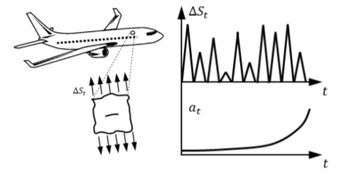


 is the Cauchy stress tensor,
  is the Kronecker delta function and
  is the strain tensor. The inputs to this parameterized model are the loading condition (the hoop stresses) and the spatial coordinates of batches of a point cloud within the computational domain. The outputs are the stresses and displacements. The network architecture consists of a Fourier feature encoding layer followed by several fully connected layers.
 : number of cycles
 and
and  : material properties (obtained through coupon tests)
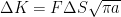
 : cyclic stresses (for example, from finite element models)
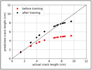
 The NVIDIA Clara AGX development kit with the us4R ultrasound development system makes it possible to quickly develop and test a real-time AI processing system for ultrasound imaging.