Imagine you’re sitting in Discord chat, telling your buddies about the last heroic round of your favorite game, where you broke through the enemy’s defenses and cinched the victory on your own. Your friends think you’re bluffing and demand proof. With GeForce NOW’s content capture tools running automatically in the cloud, you’ll have all the Read article >
Hi all, i am struggeling to get Tensorflow-Lite running on a Raspberry Pi 4. The problem is that the model (BirdNET-Lite on GitHub) uses one special operator from Tensorflow (RFFT) which has to be included. I would rather use a prebuilt bin than compiling myself. I have found the prebuilt bins from PINTO0309 in GitHub but don’t understand if they would be useable or if i have to look somewhere else. BirdNET is a software to identify birds by their sounds, and also a really cool (and free) app. Many thanks!
A one liner : For the DevOps nerds, AutoDeploy allows configuration based MLOps.
For the rest : So you’re a data scientist and have the greatest model on planet earth to classify dogs and cats! :). What next? It’s a steeplearning cusrve from building your model to getting it to production. MLOps, Docker, Kubernetes, asynchronous, prometheus, logging, monitoring, versioning etc. Much more to do right before you The immediate next thoughts and tasks are
How do you get it out to your consumer to use as a service.
How do you monitor its use?
How do you test your model once deployed? And it can get trickier once you have multiple versions of your model. How do you perform A/B testing?
Can i configure custom metrics and monitor them?
What if my data distribution changes in production – how can i monitor data drift?
My models use different frameworks. Am i covered? … and many more.
What if you could only configure a single file and get up and running with a single command. That is what AutoDeploy is!
Read our documentation to know how to get setup and get to serving your models.
AI is at play on a global stage, and local developers are stealing the show. Grassroot communities are essential to driving AI innovation, according to Kate Kallot, head of emerging areas at NVIDIA. On its opening day, Kallot gave a keynote speech at the largest AI Expo Africa to date, addressing a virtual crowd of Read article >
The transportation industry is adding more torque toward realizing autonomy, electrification and sustainability. That was a key takeaway from Germany’s premier auto show, IAA Mobility 2021 (Internationale Automobil-Ausstellung), which took place this week in Munich. The event brought together leading automakers, as well as execs at companies that deliver mobility solutions spanning from electric vehicles Read article >
Running PyCarert on GPU not only streamline model building but offsets the time cost.
PyCaret is a low-code Python machine learning library based on the popular Caret library for R. It automates the data science process from data preprocessing to insights, such that short lines of code can accomplish each step with minimal manual effort. In addition, the ability to compare and tune many models with simple commands streamlines efficiency and productivity with less time spent in the weeds of creating useful models.
This post will go over how to use PyCaret on GPUs to save both development and computation costs by an order of magnitude.
All benchmarks were run with nearly identical code on a machine with a 32-core CPU and four NVIDIA Tesla T4s. For simplicity, GPU code was written to run on a single GPU.
Getting started with PyCaret
Using PyCaret is as simple as importing the library and executing a set-up statement. The setup() function creates the environment and offers a host of pre-processing features all in one go.
After a simple setup, a data scientist can develop the rest of their pipeline, including data preprocessing/preparation, model training, ensembling, analysis, and deployment. After the data is prepared, a great place to start is by comparing models.
True to PyCaret’s ethos of simplicity, we can compare a host of standard models to see which are best for our data with a single line of code. The compare_models command trains all the models in PyCaret’s model library using default hyperparameters and evaluates performance metrics using cross-validation. A data scientist can then select the models they’d like to use, tune, and ensemble based on this info.
Figure 1: Output of the compare_models command in PyCaret.
**Models are sorted best to worst, and PyCaret highlights the top results in each metric category for ease of use.
Accelerating PyCaret with RAPIDS cuML
PyCaret is a great tool for any data scientist to have in their arsenal, as it streamlines model building and makes running many models easy. PyCaret can be made even better with GPUs. Since PyCaret does so much work behind the scenes, seemingly simple commands can take a long time. For example, we ran the commands preceding on a dataset with roughly half a million instances and over 90 attributes (UC Irvine’s Year Prediction MSD dataset). On the CPU, it took over 3 hours. On a GPU, it took less than half that.
In the past, using PyCaret on a GPU would have required many manual coding, but thankfully, the PyCaret team has integrated the RAPIDS machine learning library (cuML), meaning you can use the same simple API that makes PyCaret so effective while also using the computational ability of your GPU.
Running PyCaret on a GPU tends to be much faster-meaning you can make full use of everything PyCaret has to offer without balancing time costs. Using the same dataset just mentioned, we tested PyCaret ML functionality on both a CPU and a GPU, including comparing, creating, tuning, and ensembling models. Performing the switch to GPU is simple; we set use_gpu to True in the setup function:
With PyCaret set to run on GPU, it uses cuML to train all of the following models:
Logistic Regression
Ridge Classifier
Random Forest
K Neighbors Classifier
K Neighbors Regressor
Support Vector Machine
Linear Regression
Ridge Regression
Lasso Regression
K-Means Clustering
Density-Based Spatial Clustering
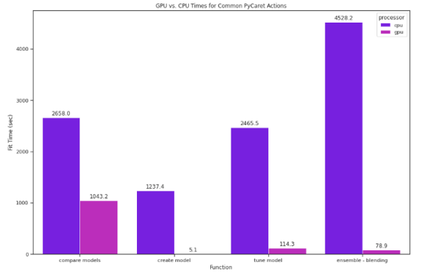
Running the same compare_models code solely on GPU was over 2.5 times as fast.
The impact was even greater on a model-by-model basis with popular but computationally expensive models. The K Neighbors Regressor, for example, was 265 times as fast on GPU.
Figure 2: Comparison of common PyCaret actions run on CPU versus GPU.
Impact
The simplicity of PyCaret’s API frees up time that would otherwise be spent coding so data scientists can do more experiments and fine-tune their experiments. When paired with GPUs, this impact is even greater, as the computation costs of taking full advantage of PyCaret’s suite of evaluation and comparison tools are significantly lower.
Conclusion
Extensive comparing and evaluating models can help improve the quality of your results, and doing so efficiently is exactly what PyCaret is for. PyCaret on GPU offsets the time costs that go along with so much processing.
The goal of RAPIDS is to accelerate your data science, and PyCaret is among a growing list of libraries whose compatibility with the RAPIDS suite can help bring a new layer of efficiency to your machine learning pursuits.
Combining mentoring, socializing, and specialized training proved key for the virtual 2021 KISTI GPU Hackathon.
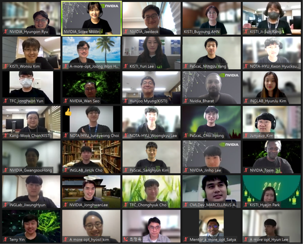
Due to the coronavirus, the 2021 Korea Institute of Science and Technology Information (KISTI) GPU Hackathon was held virtually, under the guidance of expert mentors from KISTI, NVIDIA, and the OpenACC Organization. With the goal of inspiring possibilities for scientists to accelerate their AI research or HPC codes, the hackathon provided opportunities for solving research problems and expanding expertise using NVIDIA GPU parallel computing technology.
Known for being a face-to-face event, a virtual hackathon poses its own challenges for both attendees and hosts. The new format also required juggling a diversity of teams—composed of three HPC and AI teams, four higher education and research teams, and two industry teams.
The event team found the following recipe helped create a meaningful and successful experience for the participants:
Mentoring
Based on their expertise in specific domains or programming languages, dedicated mentors were paired with teams for guidance in setting goals, and considering different approaches. The mentors collaboratively worked to solve problems and troubleshoot obstacles the teams encountered. Daily mentor sync-up calls each day kept everyone focused and working toward the best strategy for meeting their goals.
Figure 1. KISTI GPU Hackathon 2021.
Socializing
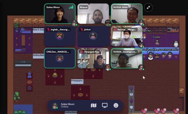
Everyone knows that all work and no play can actually hinder a team’s productivity. The hackathon provided a TGIF social hour session for participants and mentors. Using the Metaverse Gather Town Space, mentors and teams shared experiences, recharged their batteries, and developed connections that helped them continue forward for the duration of the event.
Figure 2. The TGIF social hour.
Resources and Live Seminars
Another important ingredient to success was making specialized training and resources available to attendees. For example, an NVIDIA Deep Learning Institute (DLI) workshop covering CUDA C/C++ topics was presented by a DLI ambassador and mentor. Other mentors provided team-dedicated tech sessions focused on TRT and NVIDIA Triton, OpenACC, and Nsight systems for profiling, parallel computing, and optimization.
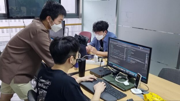
Figure 3. PaScaL team working on their project.
Hard Work Pays Off
The PasCal team from Yonsei University is developing a thermal fluid solver that efficiently calculates the thermal motion of turbulence. At this hackathon, the team converted existing code based on CPUs to a multi-GPU environment through OpenACC and cuFFT Library. This resulted in accelerating the calculations by 4.84 times RHS (right-hand side, fraction step) of one of most time consuming subroutines.
The Amore Opt team from AmorePacific cosmetics company worked on GPU optimization of DeepLabV3 + segmentation model. By applying what they learned about the TensorRT Inference optimizer and NVIDIA Triton inference server, they improved inference speed making it 26 times faster. They did this while maintaining the accuracy in their AI models to detect skin problems for their future large-scale customer service.
Video 1. TFC Team interview for KISTI Hackathon.
The TFC team from Seoul National University joined a project to accelerate a CPU-based Fortran in-house fluid calculation code. By using NVIDIA GPUs at KISTI, the team accelerated the time-consuming Tri-Diagonal Matrix Algorithm (TDMA) for thermal solver and momentum solver and Fast Fourier Transform (FFT) for pressure solver calculations. They achieved a speed 11.15 times faster on a single V100 GPU.
NVIDIA Inception member Nota and HangYang University teamed-up to optimize the Nota Model compression engine by leveraging the Tensor Core in NVIDIA GPUs for INT4 quantization. Named NOTA-HYU, the team learned to use NVIDIA profiling tools Nsight system and Nsight Compute. They then applied NVIDIA library CUTLASS to achieve an overall speed 1.85 times faster for their residual block with CUDA optimization.
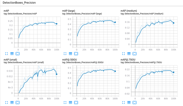
I just started using Tensorflow and Keras not long along ago, and I really like the field of deep learning. Right now I am doing it as more of a hobby than anything, and I recently learned about the concepts of transfer learning and fine-tuning. I tried to apply them to a dataset of microscopic images using the tutorial here: https://www.tensorflow.org/tutorials/images/transfer_learning.
I am using ResNet50 with the ImageNet weights, but am far from getting good results. I think it might be because of the learning rate OR because of the activation function in my last layer OR because of the fact that I use the Adam optimizer and not SGD.

 Running PyCarert on GPU not only streamline model building but offsets the time cost.
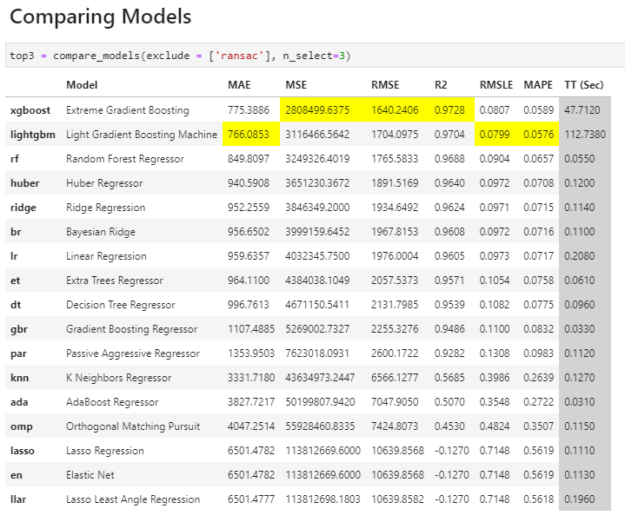
 Combining mentoring, socializing, and specialized training proved key for the virtual 2021 KISTI GPU Hackathon.