Simulations are pervasive in every domain of science and engineering, but they often have constraints such as large computational times, limited compute resources, tedious manual setup efforts, and the need for technical expertise. Neural networks not only accelerate simulations done by traditional solvers, but also simplify simulation setup and solve problems not addressable by traditional … Continued
Simulations are pervasive in every domain of science and engineering, but they often have constraints such as large computational times, limited compute resources, tedious manual setup efforts, and the need for technical expertise. Neural networks not only accelerate simulations done by traditional solvers, but also simplify simulation setup and solve problems not addressable by traditional solvers.
NVIDIA SimNet is a physics-informed neural network (PINN) toolkit for engineers, scientists, students, and researchers who are getting started with AI-driven physics simulations. You may also be looking to leverage a powerful, existing framework to implement your domain knowledge and solve complex nonlinear physics problems with real-world applications.
A success story of SimNet’s application today is in the use of hybrid PINNs for digital twins in prognosis and health management. This effort was led by Prof. Felipe Viana, an assistant professor at the University of Central Florida. He leads the group’s research in state-of-the-art probabilistic methods fusing physics-based domain knowledge and multidisciplinary analysis and optimization with applications in design, diagnostics, and prognostics.
Aircraft use case study
Maintenance of engineering assets and industrial equipment (such as aircraft, jet engines, wind turbines, and so on) is critical for safety as well as enhanced profitability in the services and warranties of these assets. Effective preventive maintenance requires the knowledge of the various operating parameters and their impact on the wear and tear of equipment. Simulations, advanced analytics, and deep learning algorithms enable the predictive modeling of complex systems and their operating environment.
Unfortunately, building models that estimate residual useful life for such equipment in large fleets is daunting. This is due to factors such as duty cycle variations, harsh environments, inadequate maintenance, and mass production problems that cause discrepancies between designed and observed component lives.
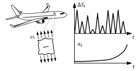
In this research project, Prof. Viana and his team of researchers built predictive models for fatigue crack growth prognosis on aircraft window panels (Figure 1), where models were trained using historical flight records (origin and destination airports, cruise altitude, and so on) and limited inspection observations (such as the crack length data for only a portion of the fleet, and so on). When the model was built and validated, it was then applied in a fleet of 500 aircraft to analyze the success of the model on larger data sets. Such predictive models are also called digital twin models and they have been increasingly used in prognosis and health management applications of industrial equipment.
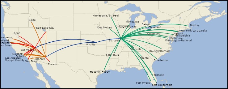
Based on literature and freely available data, synthetic data for a representative fleet of 500 narrow-body aircraft was created. The fleet is equally divided into 10 route structures (Figure 2). Each aircraft flies an average of five flights per day.
After four years of operation, the fleet starts being inspected. At this point, consider a case in which after inspecting 25 aircraft, the operator finds that some exhibit fatigue cracks at the corner of a given window. These cracks happen to be larger than anticipated. From a scientific standpoint, this poses the following challenge: if predictions were wrong due to model assumptions, is there a way to correct that?
The business implication is straightforward. When such a discrepancy is observed, operators must decide which aircraft to inspect next.
Assume that you have available the flight data from the fleet for the past four years. The hoop stresses that govern the fatigue crack growth are a function of the aircraft cabin pressure differential, which is a function of cruise altitude. The purely physics-based model assumes the local geometry correction factor F = 1.122. In reality, that is ultimately a function of the crack length. The digital twin for this component must be predictive and aircraft-specific, in addition to being computationally efficient.
There are two main challenges. First, the data is highly unbalanced. For the aircraft fleet that was being analyzed, there were only 182,500 input points and only 25 output points. Building purely machine learning models under such circumstance is extremely hard.
Second, while the conventional physics-based models maybe accurate, they often entail engineering assumptions regarding loading conditions. Considering that the sample size for this problem includes a fleet of 500 aircraft, these simulations must be done a few million times.
To overcome these challenges, Prof. Viana and team developed a novel hybrid physics-informed neural network model. Figure 3 shows where they performed cumulative damage accumulation based on recurrent neural networks merging physics-informed and data-driven layers.
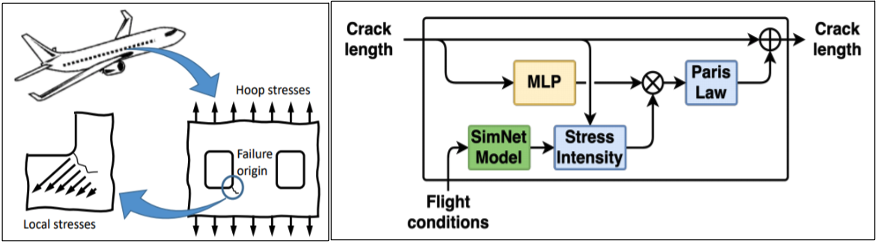
Full-fledged finite element analysis configured for crack growth simulation is extremely expensive. Therefore, it is simply not feasible for digital twin applications. This is true even if we were to run simulations for hundreds of aircraft many times over, as we optimized inspections and decided how to swap routes for a few aircraft. A parameterized physics-driven AI model is constructed in SimNet that satisfies the governing laws of linear elasticity, as follows:

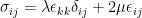

Here, 


Unlike the traditional data-driven models, no training data is used here. Instead, the loss functions are augmented by the linear elasticity laws, and the required second-order derivatives are computed using automatic differentiation. Initial and boundary conditions are also imposed as soft constraints to fully specify the physical system. Several techniques are used to enhance the accuracy and convergence speed of the model, such as network weight normalization, signed distance loss weighting, differential equation normalization and nondimensionalization, and XLA kernel fusion.
After a single training, this parameterized model provides instantaneous prediction of cyclic stresses for a variety of different loading conditions. This instantaneous prediction is critical in digital-twin applications where real-time predictions are needed. However, traditional solvers can only solve for one configuration at a time. Moreover, data-driven, surrogate-based approaches suffer from interpolation error and the predictions may not satisfy the governing laws.
For this trained parameterized model, several SimNet predictions are validated against a commercial solver, showing a close agreement with a difference of less than 5% in the maximum Von Mises stresses. Training of this model was performed on a single V100 GPU. SimNet also offers scalable performance for multi-GPU and multi-node implementation with TF32 support for accelerated convergence.
In Prof. Viana’s model, engineers and scientists can use physics-informed layers to model well-understood phenomena. This might include mechanical stress calculations to estimate the damage accumulation with Paris law fatigue increment block. Another example would be using data-driven layers to model poorly characterized parts such as corrections in stress intensity due to geometry of crack. This is where hybrid models can help estimate fatigue crack growth on fuselage panels with window cutouts.
In Figure 4, the “before training” curve uses purely physics-based models. These are obtained through numerical integration of Paris law using linear elasticity in the calculation of cyclic stresses:

: number of cycles
and
: material properties (obtained through coupon tests)
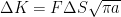

In Figure 4, the “after training” curve uses the hybrid model where the MLP layer in the RNN cell compensates for missing physics (adjusting predictions without violating the physics).
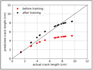
After the hybrid model is trained, we use it to predict crack length histories for the entire fleet of 500 aircraft. The 500 pressure differential time series amount for more than 3.5M data points. The hybrid cumulative damage recurrent neural network, using SimNet for stress calculations, predicts the crack length histories in 5 years. The results are illustrated in Figure 5. This enables the operators to prioritize which aircraft will be brought for inspection or swapping aircraft of different route structures.
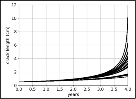
Operators could use the hybrid model to analyze the entire fleet. The results dashboard could visualize the most aggressive route structures in terms of cumulative damage rates; number of aircraft at high, medium, or low risk levels; as well which tail numbers are in which buckets (Figure 6).
In terms of actionable outcomes, operators could use the hybrid model to decide which aircraft should be brought for inspection next. They could swap aircraft between routes so that damage accumulation is mitigated while inspections are performed.
This framework handles highly unbalanced datasets formed by few output observations and data lakes containing time series used as inputs. GPU computing enables scaling up computations for fleets of hundreds of aircraft, keeping training under a few hours and inference under a few seconds.
Prof. Viana’s application’s implementation has been done in TensorFlow v2.3 using the Python APIs on various NVIDIA GPUs. Depending on the application and computing needs, you can use high-performance GPU-based clusters, a smaller Linux server with few GPUs, or even the NVIDIA Jetson. For this study, we used a Linux server with two Intel Xeon Processor E5-2683 and two NVIDIA P100 GPUs.
Next steps
In the future, Prof. Viana and his team plan on expanding the use of SimNet in their hybrid PINNs for cumulative damage by tackling even more complex applications where loading and deformation are highly nonlinear and potentially involve multiphysics. Given the flexibility of the approach, he hopes to expand the applications to other industries besides civil aviation and failure modes, such as corrosion and oxidation.
Prof. Viana elaborated on his experience. “SimNet’s accuracy is comparable to other computational mechanics software. However, its computational efficiency, quick turnaround time, and easy integration with existing machine learning frameworks makes it our choice of toolkit for our simulation needs. With SimNet, we scaled our predictive model to a fleet of 500 aircraft and get predictions in less than 10 seconds. If we were to perform the same computations using high-fidelity finite element models, we could be talking about a few days to a week. As a research institution, we see SimNet as a tool of the future where it unlocks possibilities and enables us to explore modeling approaches that were not possible before.”
For more information, see the following resources:
- Cumulative damage modeling with recurrent neural networks whitepaper
- Hybrid Physics-Informed Neural Networks for Digital Twin in Prognosis and Health Management (GTC’21 session)
- Physics-informed neural networks package GitHub repo
- Python Implementation of Ordinary Differential Equations Solvers using Hybrid Physics-informed Neural Networks tutorial on GitHub
To ask questions about Prof. Viana’s work and see what others are doing with SimNet toolkit, join the SimNet forum. For more information about SimNet’s features and to download the SimNet toolkit, see NVIDIA SimNet.
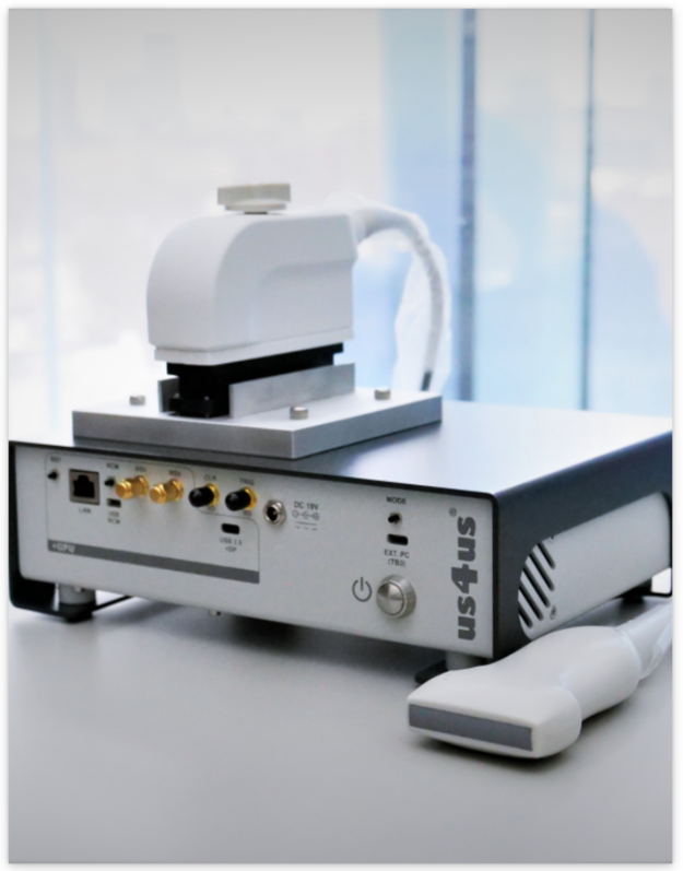
 The NVIDIA Clara AGX development kit with the us4R ultrasound development system makes it possible to quickly develop and test a real-time AI processing system for ultrasound imaging.
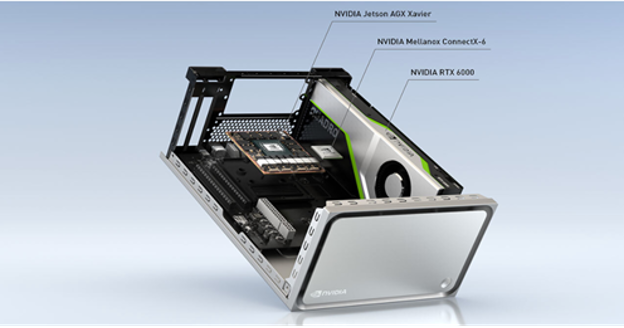


 From award-winning research demos to photorealistic graphics created with NVIDIA RTX and Omniverse, see how NVIDIA is breaking boundaries in AI, graphics, and virtual collaboration.
  Sign up for webinars with NVIDIA experts and Metropolis partners on Sept. 22, featuring developer SDKs, GPUs, go-to-market opportunities, and more.
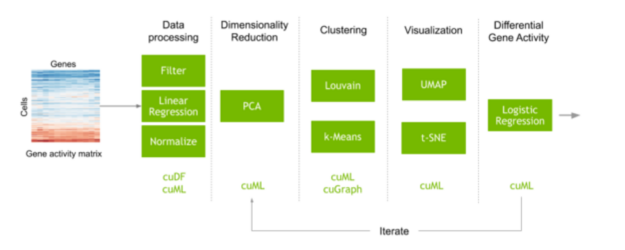
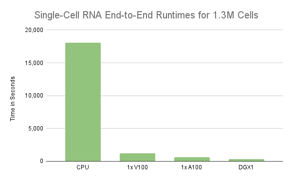
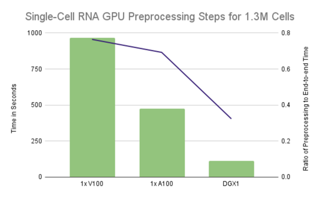
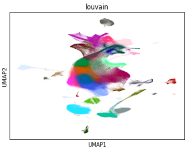
  Learn how the use of RAPIDS to accelerate the analysis of single-cell RNA-sequence on a single NVIDIA V100 GPU shows a massive performance increase.